Recommendations for visual predictive checks in Bayesian workflow

This paper is under review on the experimental track of the Journal of Visualization and Interaction. See the reviewing process.
1 Introduction
Assessing the sensibility of model predictions and their fit to observations is a key part of most model building workflows. These assessments may reveal that the model predictions poorly represent (or replicate) the observed data, prompting the modeller to either improve their model, or adjust their confidence in the predictions accordingly. In this paper, we focus on examples rising from Bayesian workflows (Gabry et al. 2019; Gelman et al. 2020), such as posterior predictive checking [PPC; Box (1980);Rubin (1984); Gelman, Xiao-Li, and Stern (1996); Gelman et al. (2013)], and visualizations of data, posterior, and posterior predictive distributions. Visualization of data distribution is useful even if we do not do any modeling. In Bayesian inference, the posterior distribution presents the uncertainty in the parameter values after conditioning on data, and the posterior predictive distribution presents the uncertainty in the predictions for new observations. The posterior inference is often performed using Monte Carlo methods (Štrumbelj et al. 2024), and posterior and posterior predictive distributions are then represented with draws from these distributions. In the same way as we visualize data distributions, we can visualize posterior and posterior predictive distributions. In posterior predictive checking, we compare the data distribution to the posterior predictive distribution. If these distributions are not similar, the model is misspecified and we should consider improving the model. These visualizations are also applicable to prior predictive checking, where one might compare prior predictive samples to some reference values rising from domain knowledge (Wesner and Pomeranz 2021), and to cross-validation predictive checking where data are compared to cross-validation predictive distributions to avoid double use of data.
The purpose of this paper is to illustrate common issues in visual predictive checking, to provide better recommendations for different use cases, and to provide diagnostics to automatically warn if useless or misleading visualization is used. Together we have decades of experience in teaching visual predictive checking and helping modellers using popular visual predictive checking tools such as bayesplot (Gabry and Mahr (2024)) and ArviZ (Kumar et al. (2019)). We have seen many times where students and modellers use commonly recommended visualizations without realizing that in their context, the specific visualization is the wrong one and either useless or even misleading. Backed up with arguments from recent studies in uncertainty visualization, we provide a summary of methods we recommend. These methods are aimed to offer an informed basis for decision-making, be it for the modeller to improve on the model or for the end user to set expectations on the performance of the model.
The visualizations we discuss should be considered as broadly-applicable tools aimed to give insight into the overall goodness of model fit to the observations, as well as to possible deviations in certain parts of the predictive density. Most modeling workflows benefit from additional visualizations tailored to their specific use cases, as there is no general visual or numeric check that would reveal every aspect of the predictive capabilities of any given model. Some commonly-used methods for visualizing model predictions have risen from comparisons of continuous variables, and as such have varying degrees of usability for assessing predictions with discrete values. Some may not work with all continuous cases, in case of sharp upper or lower bounds in the set of possible values the prediction can take.
In Section 2, we inspect the common use of kernel density estimates (KDE) in summarizing the predictive distribution and the observed data, and show comparisons between commonly used visualization approaches. We highlight common cases when these visualizations may hide useful information and propose an automated goodness-of-fit test to alert the modeller of the presence of conflict between the data and the visualization. In Section 3, we discuss the use of visualizations assuming continuous data when the data and predictions are in reality discrete, but have a high number of unique values. We also discuss an alternate way of visualizing count data, when the number of cases is large, but still small enough for the modeller to be interested in attempting to assess the predictions as individual counts. In Section 4, we focus on workflows involving binary predictions. We showcase tools that expand the visualizations beyond the typical bar graphs and binned calibration plots and instead allow for a more robust assessment of the calibration of the predictive probabilities. In Section 5 and Section 6, we show how the visual predictive checks described for binary predictions can be extended to discrete predictions with a small or medium number of individual cases.
2 Visual predictive checks for continuous data
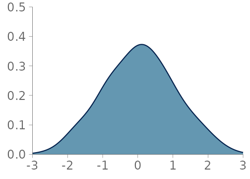
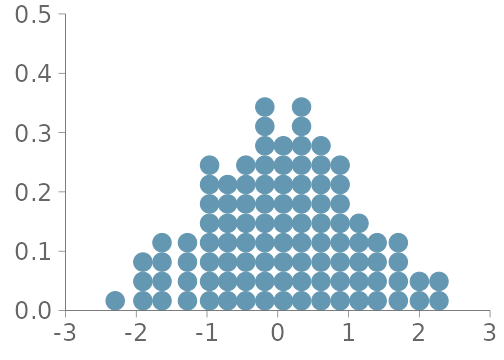
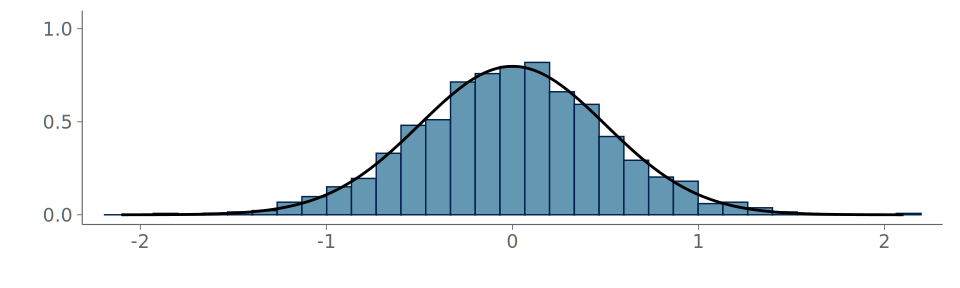
In this section, we consider visualizations for observations from a continuous or almost everywhere continuous distribution. We focus on three data visualizations; histograms, and KDE-based continuous density plots, as they are the two most commonly used visualizations for summarizing unidimensional distributions, and quantile dot plots (Kay et al. 2016) as we see that they offer a useful alternative that we recommend in many cases. Table 1 summarizes the main advantages and disadvantages of these three visualizations, and Figure 1 shows a side-by-side comparison of these visualizations. Histograms and density plots are implemented in various commonly used software packages for data visualization and are the two most common choices for initial visual PPCs (Wickham (2016); Gabry and Mahr (2024); Kumar et al. (2019); Kay (2024)).

| Visualization | Advantages | Disadvantages |
|---|---|---|
| Histogram |
|
|
| KDE plot |
|
|
| Quantile dot plot |
|
|
Histogram
Here, we consider the most commonly used histograms, which are centered over the data, and where all of the bins have an equal width (see an example in Figure 1 (a)). These bin widths are either chosen by the modeller, or through a heuristic, such as the Freedman-Diaconis rule (Freedman and Diaconis 1981). Often, instead of choosing the bin width directly, the modeller inputs a desired amount of bins and an equal partitioning of the data range is computed with an adequate number of breaks.
KDE-based density plot
The most typical KDE-based density plot, often simply called a density plot, is a line or filled area representing a density approximation obtained through convolution of the data with some kernel function (see an example in Figure 1 (b)). Most commonly, a Gaussian kernel is used for the approximation, and a kernel bandwidth is selected through one of the widely used algorithms (Sheather and Jones 1991; Scott 1992; Silverman 2018). As the default implementation of the KDE plot in most visualization software packages is usually enough to produce aesthetically pleasing smooth summaries of the data, KDE plots are a very popular method of visually summarizing data.
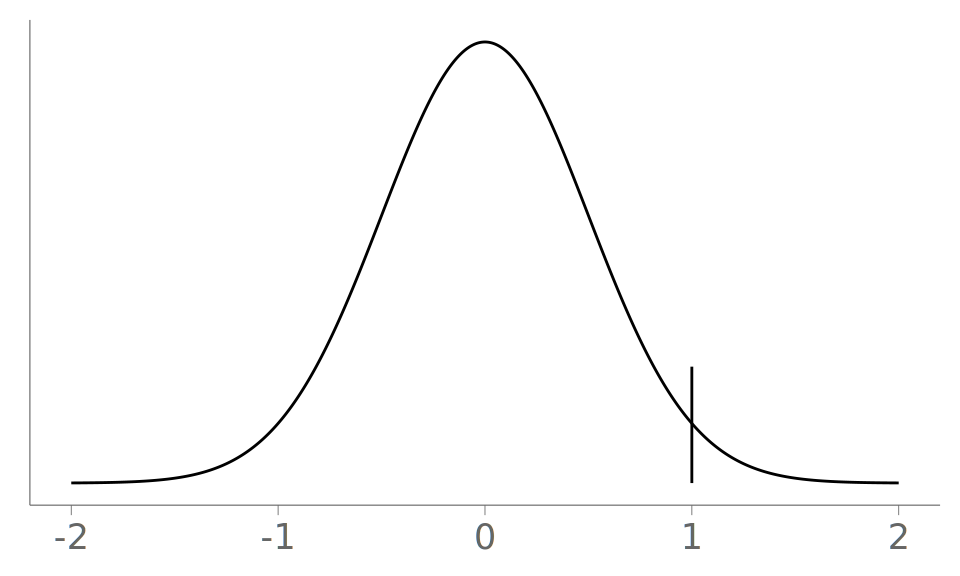
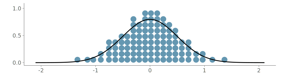
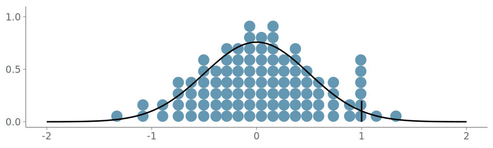
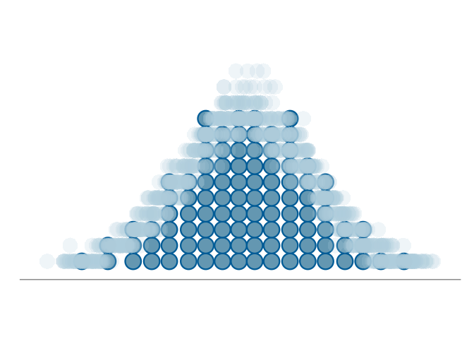
Quantile dot plot
The quantile dot plot (Kay et al. 2016), is a dot plot, where a set number of the observed quantiles—we use one hundred—are visualized instead of the observations themselves (see an example in Figure 1 (c)). This results in a visual density estimator with a low bias and high variance similar to that of a histogram (Wilkinson 1999). Kay et al. (2016) show that a quantile dot plot with one hundred quantiles performs very similarly to a KDE-based density plot for tasks of estimating probabilistic predictions from visualizations. Compared to KDEs, quantile dot plots have the added benefit of allowing for fast visual probability estimation in the tails of the distribution. In our experience, and as shown in Section 2.6 and Section 2.4 in case of discontinuities and outliers, quantile dot plots also offer a better visualization than kernel density plots and histograms.
Advantages and disadvantages of the three visualizations
In Table 1 we have collected what we see as the main advantages and disadvantages of histograms, KDE density plots, and quantile dot plots for visualizing observations and assessing the quality of model predictions. Both the histogram and the KDE density plot have commonly recognized drawbacks, summarized by a trade-off between over and under smoothing.
The choice of bin width and breakpoints causes histograms to suffer from binning artefacts (Dimitriadis, Gneiting, and Jordan 2021). Additionally, comparing the histogram of observations to multiple histograms visualizing predictive samples may be difficult.
Density plots from KDEs, as shown in Section 2.4, Section 2.5, and Section 2.6, have a tendency to either hide details such as discontinuities in the observation distribution if the chosen bandwidth is too large, or over-fit to the sample when the bandwidth is too small. When over-fitting, comparing multiple density plots may be difficult, as there is more variation on the estimate of the underlying distribution. These drawbacks are typically especially common in the standard implementations of KDE density plots. More specialized software often implement measures, such as automated boundary detection and less conservative bandwidth selection algorithms, to mitigate these issues (Kumar et al. 2019; Kay 2024).
Based on our experience, we prefer quantile dot plots in many cases, as they offer a low overhead solution to plotting the data without defining a suitable binning and are flexible enough to represent distributions with long tails.
Assessing the goodness-of-fit of a density visualization
As KDE plots, histograms, and quantile dot plots all produce a visualization of a density, we can assess the representativeness of the visualization by assessing the goodness-of-fit of the implied density estimate to the data being visualized. To assess the goodness-of-fit of a density estimate \hat f, we test for the uniformity of the probability integral transformed (PIT) data \lbrace x_1,\dots, x_N\rbrace when the density approximator is used for the transform. The PIT value, u_i, of x_i w.r.t. a density estimator \hat f is defined as the cumulative distribution value, u_i = \int_{-\infty}^{x_i}\hat f(x)\,dx. \tag{1}
The underlying principle of this goodness-of-fit test is that, when computed with regard to the true underlying density f s.t. x_i \sim f, the PIT values would satisfy u_n \sim \mathbb U(0,1), where \mathbb U(0,1) is the standard uniform distribution.
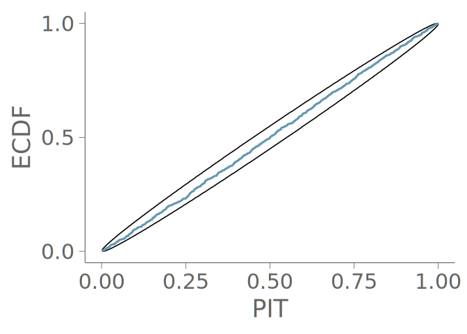
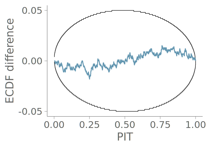
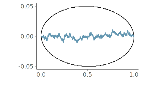
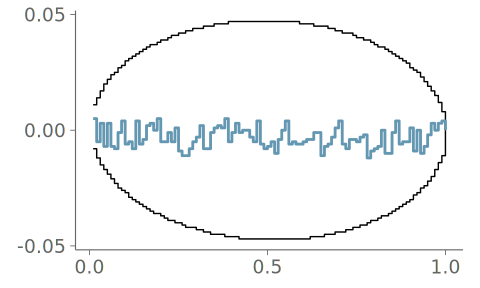
Our uniformity test of choice, due to its graphical representation that further enhances the explainability of the results, is the graphical uniformity test proposed by Säilynoja, Bürkner, and Vehtari (2022). This test provides simultaneous 1 - \alpha level confidence bands for the uniformity of the empirical cumulative distribution function (ECDF) of the PIT values. In the graphical test, the PIT-ECDF and the simultaneous confidence intervals are evaluated at a set of equidistant points along the unit interval. An example of these simultaneous confidence intervals for the ECDF of the PIT values, F_{\text{PIT}} is provided in Figure 3 (b). Alternatively, Figure 3 (c) shows the ECDF difference version of the same information, that is, the vertical axis of the plot is scaled to show the difference of the observed ECDF to the theoretical expectation, F_{\text{PIT}}(x) - x. Especially for large samples, this transformation allows for an easier assessment of the values near the ends of the unit interval.
As goodness-of-fit testing does not greatly increase the computational cost of constructing the visualizations, we propose implementing automated testing and recommendations for users to consider alternative visualization techniques when the fit of the chosen visualization isn’t satisfactory.
Next, we introduce how PIT can be implemented for the three visualizations.
PIT for KDE density plots
In theory, a KDE defines a proper probability distribution, and the PIT could be directly computed as in Equation 1. However, in practice the KDE density visualizations are often showing a truncated version of the KDE, limited to an interval centered around the domain of the observed data. For PIT computation, we limit the integration to the displayed range and normalize the results to make the truncated KDE integrate to one.
Most software implementations evaluate the KDE on a dense grid spanning the domain of the observed data, thus allowing numerical PIT computation by extracting the density values on these evaluation points and carrying out the aforementioned normalization to obtain PIT values.
PIT for histograms
For a histogram with equal bins of width h, we define the PIT as
\begin{align} \text{PIT}(x) = h\sum_{j=1}^{J} f_j + (x - l_{J+1})f_{J+1}, \end{align}
where J = \max_j \lbrace r_j \leq x\rbrace, and l_j and r_j are the left and right ends of the jth bin.
Again, the relative densities and boundaries of these bins are usually readily available in the software used for constructing these visualizations, and thus implementing the transform for histograms is a relatively simple task.
PIT for quantile dot plots
As the quantile dot plots are discrete, the PIT values computed according to Equation 1 are not guaranteed to be uniformly distributed. As demonstrated by Früiiwirth-Schnatter (1996), for a discrete random variable X, one can employ a randomized interpolation method to obtain uniformly distributed values,
\begin{align} u(x) = \alpha P(X \leq x) + (1-\alpha) P(X \leq (x - 1)), \end{align} where \alpha \sim \mathbb U(0,1).
For quantile dot plots, where n_q is the number of quantiles, c_k the horizontal position of the center of the kth dot and r the radius of the dots, we define a randomized PIT as
\begin{align} \text{PIT}(x) \sim \mathbb U\left(\frac{l(x)}{n_q}, \frac{u(x)}{n_q}\right) , \end{align}§
where n_q is the amount of quantiles, that is, dots, in the plot, and l(x) and u(x) are the quantile indices satisfying
\begin{align} u(x) = \min\lbrace k \in \{1,\dots,n_q\} \mid x < c_k - r\rbrace, \end{align}
and
\begin{align} l(x) = \begin{cases} 0,&\quad\text{if }u(x) = 1,\\ \min\lbrace k \in \{1,\dots,n_q\} \mid |c_k - x| \leq r\rbrace,&\quad\text{if }\exists \, k \text{ s.t. } |c_k - x| \leq r,\\ \max\lbrace k \in \{1,\dots,n_q\} \mid x \geq c_k - r\rbrace,&\quad\text{otherwise}. \end{cases} \end{align}
That is, we consider the left and right edges of the dots, c_k - r, and c_k + r respectively. Now the PIT value of x is limited from above by the smallest quantile dot fully to the right of x. The lower limit of the PIT value is determined in three cases. First, for those x that are to the left of all of the quantile dots, the lower limit of the PIT value is zero. Second, if x lies between the left and right edges of one or more quantile dots, the lower limit is determined by the smallest of these quantiles. Finally, when x is not between the edges of any single quantile dot, the largest dot fully to the left of x determines the lower limit of the PIT value.
Again, as the centre points and radius of the dots are required for constructing the visualizations in the first place, implementing the PIT computations is relatively straightforward.
Continuous valued observations
When the observation density is smooth and unbounded, and the practitioner uses visualizations aimed at continuous distributions, misrepresenting the data is less common. The main benefit of goodness-of-fit testing for visualizations arises, when the assumptions in the visualization do not meet the properties of the underlying observation distribution. Sometimes data, that may seem continuous at first glance, proves problematic for KDEs to visualize.
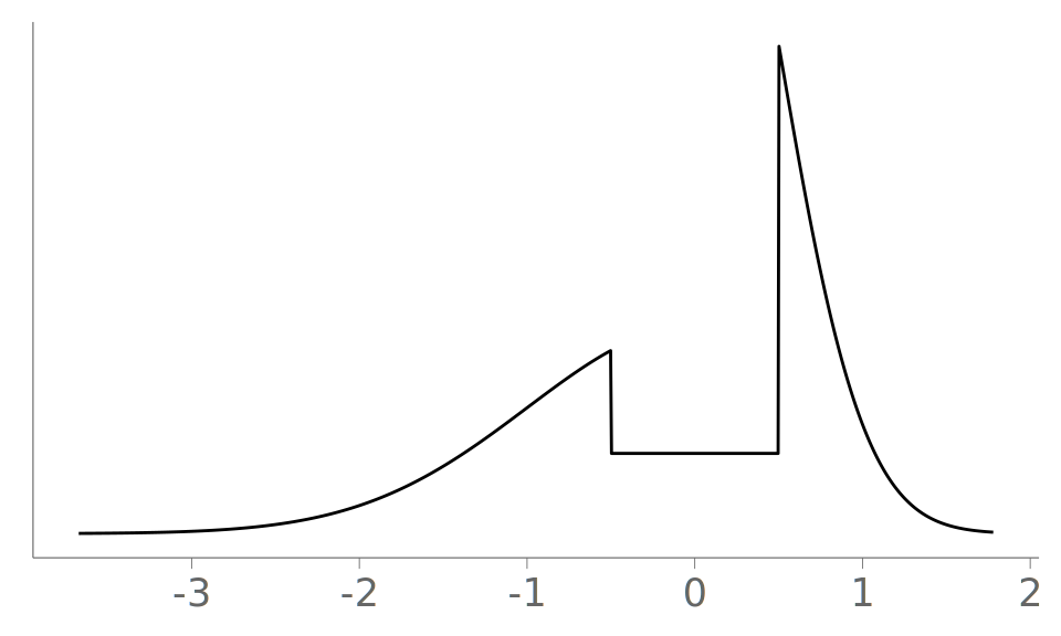
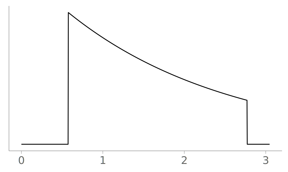
Below, we will first look at the ideal case of a continuously valued observation with a smooth and unbounded underlying distribution, and then step through three examples of continuous valued observations where the observation distribution is not smooth and visualizing the observation requires extra attention. The true underlying densities are visualized in Figure 2. In the three later cases, using the default KDE plot or histogram can hide important details of the observation, and looking at the issues detected through goodness-of-fit testing could affect future modeling choices.
Smooth and unbounded density
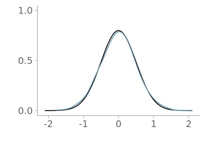
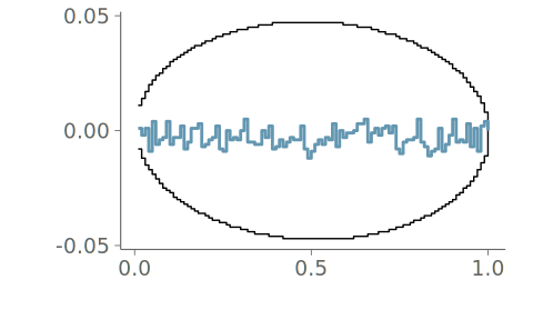
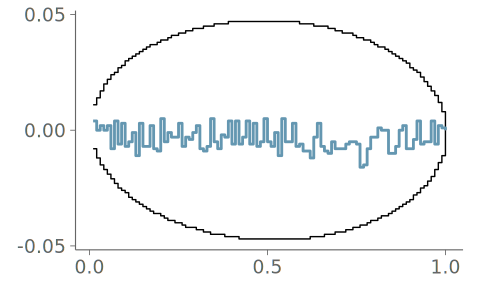
When the underlying distribution is smooth and unbounded, large issues in goodness-of-fit of the discussed three visualizations are rare. Figure 3 (a) includes the KDE plot for an observation of 1000 standard normally distributed values. Figures Figure 3 (b) and Figure 3 (c) show the corresponding goodness-of-fit test with the PIT ECDF values well within the 95% simultaneous confidence intervals for uniformity. Figure 4 shows the histogram and the corresponding goodness-of-fit assessment of the same data. This time, we show only the ECDF difference version of the graphical test. Again, no issues are detected. Figure 5 in turn shows the quantile dot plot paired with the corresponding goodness-of-fit evaluation. Again, no issues are detected. Although one hundred evaluation points results in a quite smooth visualization, the discreteness of the PIT ECDF of the quantile dot plot is visible.
Density with steps
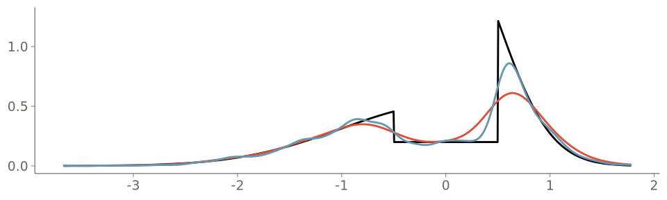
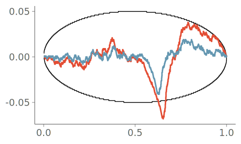
When the observation density has steps, that is, points with unequal one-sided limits, the continuous representation offered by KDEs—that assume smooth density—may struggle to accurately represent the discontinuity. In turn, the visualizations provided by histograms and quantile dot plots are more flexible, but if the location of the step is not known, an unfortunate histogram binning may introduce large deviations to the true density values. If the location of the step was known, a good representation could also be obtained with KDE plots or histograms by using separate bounded KDEs for the two sides of the step (see Section 2.5), or by tailoring the histogram by aligning the discontinuity to the boundary of two adjacent bins.
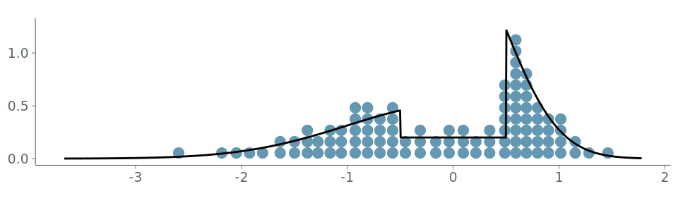
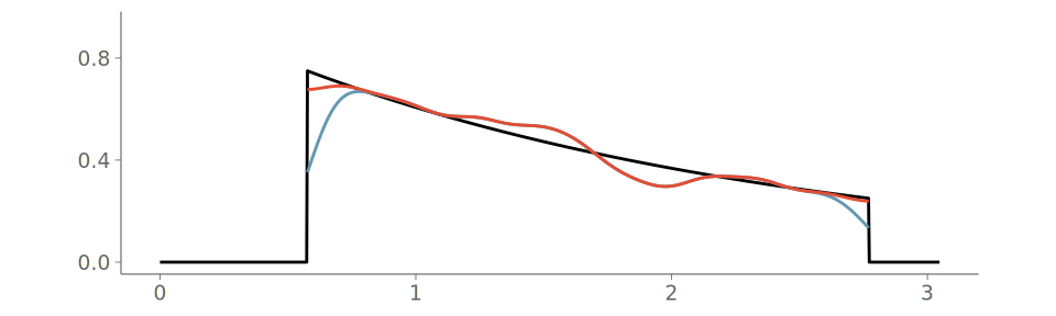
To illustrate the challenges of visualizing observations from stepped densities, we use samples from the following true density f, shown in Figure 2 (a):
\begin{align} f(x) = \begin{cases} \frac{2}{5}\Phi(-\frac{1}{2})^{-1}\mathcal{N}(x\mid 0,1), & x \leq -\frac{1}{2}\\ \frac{1}{5}, & -\frac{1}{2} < x \leq \frac{1}{2}\\ \frac{2}{5}\Phi(-\frac{1}{4})^{-1}\mathcal{N}(x\mid 0,\frac{1}{4}), & x > \frac{1}{2}, \end{cases} \end{align}
this kind of bimodal skewed distribution with low density between the modes is present for example in the z-scores of published p-values (Van Zwet and Cator 2021).
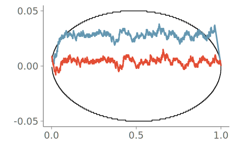
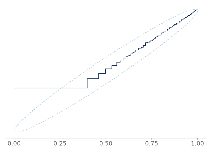
Figure 6 shows the resulting density plot and the corresponding calibration for two common kernel bandwidth selection strategies; Silverman’s rule of thumb (Silverman 2018), and the Sheather-Jones (SJ) method (Sheather and Jones 1991). Of these, SJ is expected to give a more robust bandwidth selection to data from non-Gaussian distributions (Sheather and Jones 1991). Despite this, Silverman’s rule of thumb is the default strategy in many KDE density visualization implementations using Gaussian kernels. As seen in the figure, both strategies have difficulties representing the discontinuity in the observation density, and PIT ECDF for the KDE plot using Silverman’s rule of thumb crosses the 95% simultaneous confidence interval and is recognized as having significant goodness-of-fit issues.
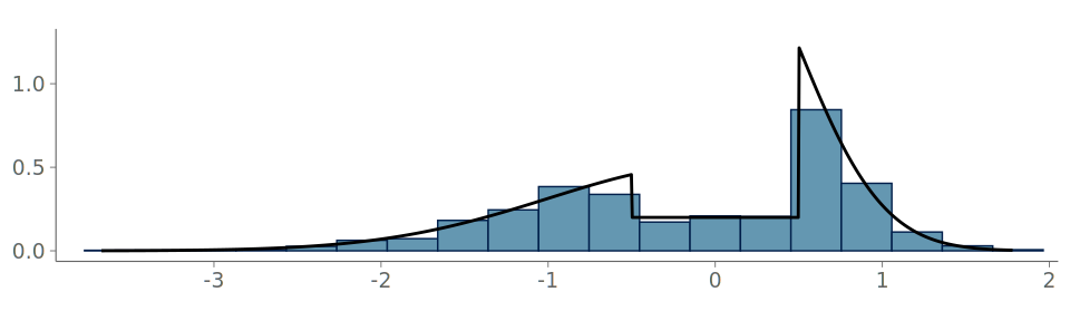
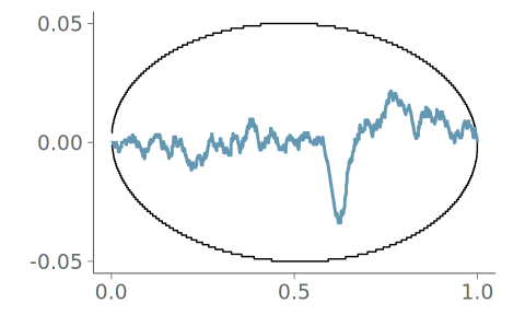
Figure 7 shows the visualization and goodness-of-fit assessment for the same data, when using a histogram. Although the discontinuity is strongly hinted in the histogram, it is not located close to a bin boundary and causes significant goodness-of-fit issues as too much density is placed on the last values of the low density region preceding the discontinuity.
Lastly, Figure 8 shows the same process for a quantile dot plot. Again, the discontinuities are visible in the plot. Here, as the visualization follows the ECDF quantiles, the discontinuities don’t cause issues to the goodness-of-fit.
Density with strict bounds
Bounded density functions are very commonplace, and a special case of the stepped densities discussed above. If the data is known to be bounded, the knowledge allows for specialized visualizations; for example, KDE plots with boundary corrections methods, such as boundary reflection, or limiting the histogram bins to the domain of the density.
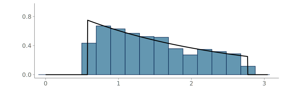
A problem arises, when unknowingly visualizing bounded data. Below, we inspect our three visualizations of interest applied to data from a truncated exponential distribution with rate parameter \lambda = 1 (shown in Figure 2 (b)). The truncation is to the central 80\% interval of the untruncated distribution.
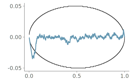
Figure 9 shows a comparison between two KDE plots; one without any information on the boundedness of the data, the other made using boundary reflection based on bounds estimated through an automated boundary detection algorithm implemented in the ggdist R package (Kay 2024). The goodness-of-fit test clearly indicates that the density is misrepresented near the boundaries by the unbounded KDE plot. In general, a \cap-shaped PIT ECDF plot indicates bias towards too small PIT values, and the strong upward trend at small PIT values indicates that the estimated density at the left tail is lower than expected if the data was sampled from the estimated density.
Figure 10 shows the data visualized with a histogram without limiting the bins to lie inside the bounds. Again, bins overlap the discontinuities, causing the goodness-of-fit test to indicate possible data misrepresentation.
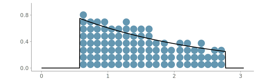
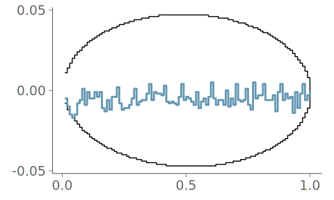
Figure 11 shows the data visualized with quantile dot plot using 100 quantiles. As the quantile dot plot by design isn’t placing any dots outside the data range, the goodness-of-fit is satisfactory.
Density with point masses
The final example of continuous valued observations with discontinuities in the density is met when one or more point masses are present. These kinds of observation densities are often met in biomedical and economical studies, where zero-inflated, but otherwise continuous data is common (Liu et al. 2019). Another cause of point masses can be problematic treatment of missing values, where any missing fields in multidimensional observations are replaced with some predetermined value, be it zero or some summary statistic.
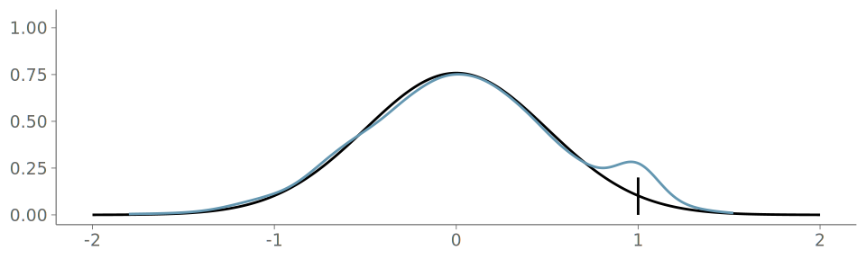
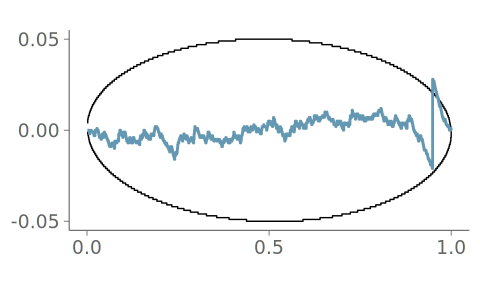
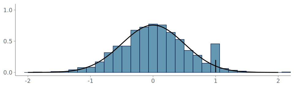
Below, we inspect an example following the density depicted in Figure 2 (c), where an observed value from the standard normal distribution is replaced with 1 with probability 0.2.
Figure 12 shows the KDE plot and the corresponding goodness-of-fit assessment, when the SJ method is used for bandwidth selection. Although the point mass does show as an additional bump in the density, the goodness-of-fit test notices that the KDE isn’t flexible enough and alerts us of the underlying point mass with a sharp jump in the PIT ECDF.
Figure 13 shows the same data visualized using a histogram. Now the discontinuity is arguably more visible in the visualization, but, as all the bins are of equal width, the PIT ECDF shows a sharp discontinuity.
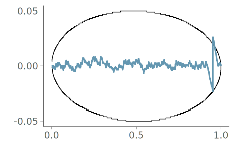
Figure 14 shows the data visualized with quantile dot plot using 100 quantiles. Again, the point mass is visible in the visualization, and the PIT ECDF indicates that the visualization is representative of the sample.
Detecting if observation is discrete or mixture of discrete and continuous
In addition to the aforementioned goodness-of-fit test, a fast and simple to implement method is to simply count unique values in the observed data. Relatively high counts of repeated values can inform the practitioner if the observations are discrete or contain point masses, for example, zero-inflation.
If at least one non-unique value, we move to check for relative frequencies of repeated values. If the relative frequency of any value is more than 2% of the full sample, we consider the possibility that the data might contain discrete values.
Visual predictive checking with overlaid plots
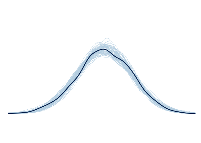
When comparing data and model predictions, one approach is to show visualization of data and visualization of the draws from the predictive distribution overlaid in one plot. The most common approach is to plot overlaid KDE plots, as it is usually easy to distinguish several overlaid KDE lines from each other. The bandwidth selection plays an important role in the comparison. On one hand, if the chosen bandwidth is narrow, the KDEs can show large variation even when repeatedly drawing from the same distribution. On the other hand, with a wide bandwidth, the KDE may be too smooth and hide important details. With histograms, and quantile dot plots, overlaid plots are rarely used, as the bin boundaries and dot locations depend on the model prediction and the resulting overlaid figure becomes difficult to read. A common solution for histograms, shown later in Section 3, is to use a shared set of bins for the predictions and data, and to increase readability by only show the predictions through per bin summary statistics, such as mean and quantile based intervals. A drawback with this approach is, that the per bin summaries don’t show dependency between the bins, making it harder to assess the global shape of the density. To compare multiple quantile dot plots to a reference plot, we propose overlaying the reference plot with just the top dots of each stack in the quantile dot plots of the predictive samples. Figure 15 (c) shows the resulting plot, which illustrates the variation in the overall form of the predictive distribution. Again, when summarizing the quantile dot plots of the predictive draws, we lose information on the dependency between heights of the stacks and the overall shape of the predictive density.
Overlaid KDE plots are usually easy to interpret—assuming the smoothness assumptions match the underlying data and draws from the predictive distribution—although they lack a quantification for when the differences are significant. For better quantification of the difference and more robust behavior in the case of non-smooth underlying distributions, we recommend the use of the graphical PIT-ECDF test described in Section 2.1. In posterior predictive checks, we assess the fit between the observations and the predictive distribution of the model. The predictive distribution is not expected to give an exact match, for example the posterior predictive distribution of a Bayesian model usually has thicker tails than the true underlying observation distribution. To avoid using the same observations for both fitting the model and assessing the predictive performance, we use leave-one-out cross-validation (LOO-CV). Especially flexible models and small observations require LOO-CV for more reliable PIT values. If one were to not use cross-validation, the PIT values would tend to be too close to 0.5 and the PIT ECDF plot would be S-shaped, suggesting many observations are too close to their respective predictive means. For fast LOO-CV computation, we recommend using Pareto smoothed importance sampling (PSIS) (Vehtari et al. 2024), estimates the leave-one-out predictive distributions without the need for refitting the model for each left out observation. In our experience, the PIT ECDF plots of both the posterior predictive and LOO-predictive draws are useful for assessing that the predictive distribution of the model is well calibrated and the visualizations give insight to the nature of the possible issues in model fit.
3 Visual predictive checks for count data
In this section, we focus on count data, which although being discrete, can benefit from both continuous and discrete visualizations. Continuous visualizations are commonly used for count data and they can sometimes be a good choice, but there are cases where they can be misleading and visual predictive checks designed specifically for count data should be used.
In predictive checking for count data, we focus on two visualizations; the overlaid KDE plots introduced in Section 2.7, and our version of the rootogram (Kleiber and Zeileis 2016). In our experience, the higher the number of distinct counts being visualized, and the smaller the variance of probabilities of individual counts is, the more effective KDEs are for visualizing count data, although one should pay close attention to the effect of the boundedness on the KDE fit as count data is usually limited to non-negative values and sometimes also has maximum count limit. Rootograms offer a visualization which emphasizes the discrete nature of the predictive and observation distributions. In our experience, rootograms are good for predictive checking of count data, when the number of distinct counts is low or there is a sharp changes in the probabilities of consecutive counts, for example, when the data exhibits zero-inflation (the probability of 0 is much higher than the probability of 1).
In Section 3.1 we show how, similarly to the cases in Section 2, goodness-of-fit tests can be used to assess how well the KDE plot represents the data. In Section 3.2 we introduce our version of the rootogram, and demonstrate its use when the familiar KDE exhibits goodness-of-fit issues. The visual predictive checks in both Section 3.1 and Section 3.2 follow an example from a modeling workflow of estimating the effect of integrated pest management on reducing cockroach levels in urban apartments (Gelman, Hill, and Vehtari 2020). We focus on assessing the quality of the predictions of a generalized linear model with a negative binomial data model for the number of roaches caught in traps during the original experiment.
Visualizing count data with KDE plots
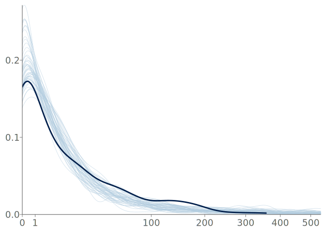
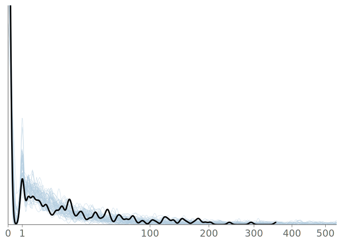
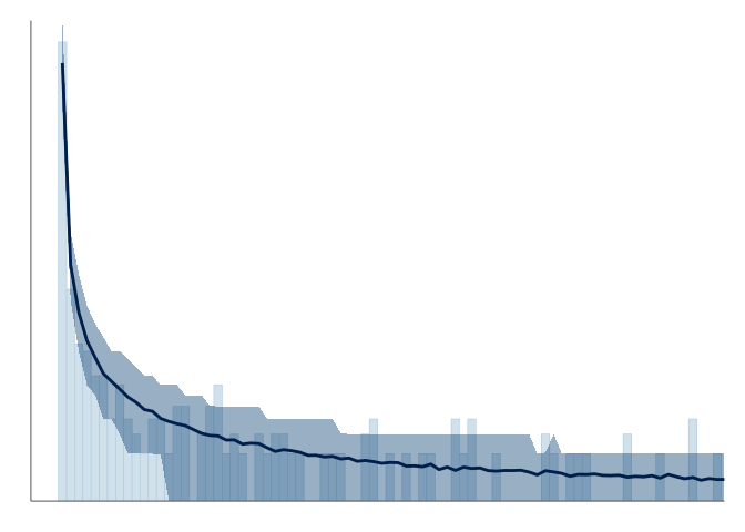
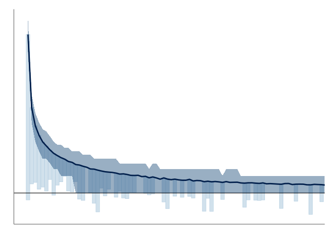
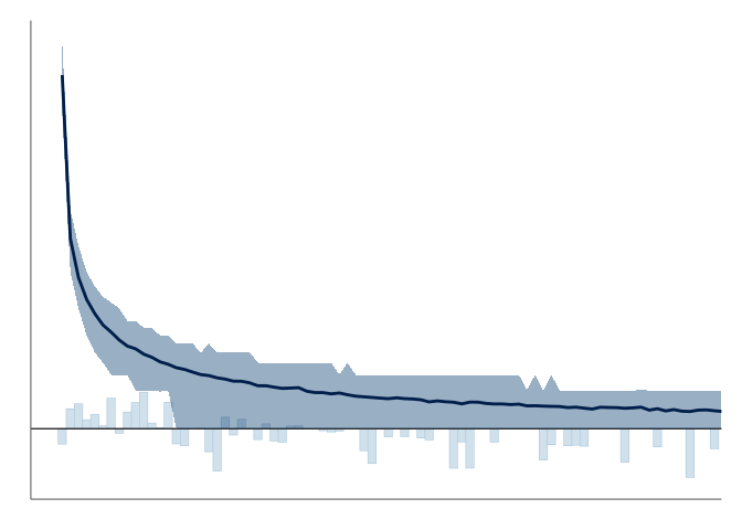
A common approach for count data, especially when the number of unique discrete values is high, is to assume that the values can be visualized as if they were from a continuous distribution. This enables the use of overlaid KDE plots for visual predictive checks. Figure 16 and Figure 17 illustrate how—after changing the default bandwidth algorithm—a KDE plot can have a satisfactory goodness-of-fit to discrete data, and how the PIT ECDF diagnostic can be used to assess the goodness-of-fit of the continuous visual representation of the discrete data.
The data in the roach dataset exhibits zero-inflation, and the default algorithm of the selected visualization software fits an unbounded KDE with a relatively large bandwidth, resulting in a bad fit shown in Figure 16. After using a left bounded KDE and the SJ bandwidth selection method, we see in Figure 17 that away from zero, the observation distribution is well summarized by the KDE plot.
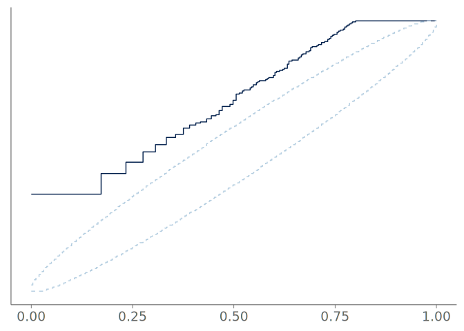
bayesplot, and is not bounded and has a relatively large kernel bandwidth. The PIT ECDF shows that the visualization assigns too much probability mass to small counts, and between the discrete integer valued observations, resulting in the PIT ECDF staying above the simultaneous confidence bands.
A reasonable step in the visual predictive checking for the roaches model, is to separate the analysis of the long tail and the bulk of the distribution. One possible approach for analyzing the tail of the distribution, is to compare how the estimated Pareto shape parameter of the predictive draws compares to the tail shape of the data. When comparing the tail shapes, one shouldn’t expect an exact fit, as the predictive distributions typically exhibit thicker tails due to uncertainty. When moving to analyze the bulk of the distribution, we see that the number of distinct counts below 90% quantile is relatively small, 48, and thus we may expect a discrete visual predictive check to perform well.
Rootograms emphasize discreteness of count data
Kleiber and Zeileis (2016) proposed rootograms to be particularly useful in diagnosing issues, such as over-dispersion and excess zeros, in count data models.
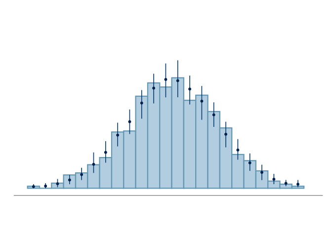
Traditionally, in a rootogram the frequencies of the observed counts are visualized with a bar plot, and predictive expected frequencies as a connected line plot. Importantly, the frequencies on the vertical axis are plotted on a square root scale to emphasize counts with low frequencies, occurring often in the tails of the distribution (see for example, Tukey 1972; Kleiber and Zeileis 2016). As shown in Figure 18 (a), one can include the visual representations of the predictive uncertainty without overly complicating the visualization. Aside from the standing rootogram in figure Figure 18 (a), two common variations are the hanging and suspended rootogram, shown in Figure 18 (b) and Figure 18 (c) respectively. These alternatives offer a more pattern focused approach to inspecting the possible differences between the observed and predicted values.
In the hanging rootogram, the observed frequencies are drawn hanging form the predictive mean, placing the lower end of the bar at the difference of the predicted mean and the observation, y_{pred} - y_{obs}. This end is then directly readable as over- or underestimation, depending if the bar is above or below the horizontal axis.
The suspended rootogram instead visualizes the residual, y_{obs} - y_{pred}, as bars with their other end at the horizontal axis of the visualization.
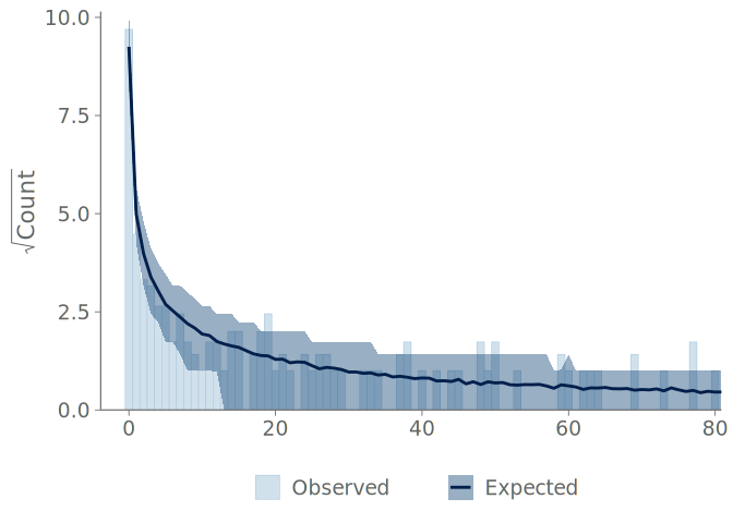
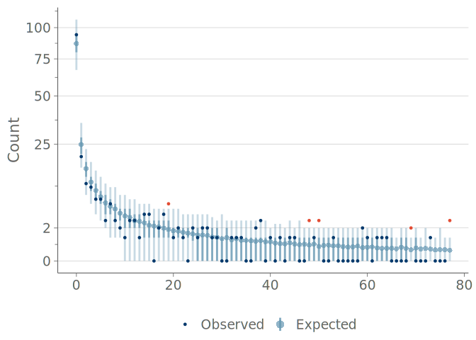
Figure 19 (b) shows our proposed modification to the traditional rootogram. This version has two main differences to the previously used visualizations; first, it emphasizes the discreteness of the predictions by showing the predictive frequencies as points and point-wise credible intervals, instead of connecting these into lines and filled areas. For overlaying, we prefer to show the observations as points and use color to highlight the observations falling outside the credible intervals. Although some values are expected to fall outside the credible intervals, these are often of interest to the practitioner for identifying possible issues. The second important distinction is how we implement the square root scaling on the vertical axis—instead of the traditional method of having an axis with equally spaced tick marks displaying the square roots of the frequencies—we transform the axis to square root scale and display the untransformed frequencies (see comparison in Figure 19). We recommend the use of axis ticks or horizontal lines as visual cues of the non-linear scaling. This second change allows for a more natural reading of the frequencies shown on the vertical axis of the plot.
4 Visual predictive checks for binary data
Assessing the calibration of binary predictions is a common task made difficult by the discreteness of the observed outcome. Below, we walk through two usual approaches, and introduce an alternative offered by PAV-adjusted calibration plots (Dimitriadis, Gneiting, and Jordan 2021).
We continue using the roaches example introduced in Section 3, and consider three models for predicting if one or more roaches will be observed:
- an intercept-only model estimating the overall probability of observing one or more roaches,
- the negative binomial regression model from Section 3.
- a zero-inflated version of Model 2 using the covariates to additionally model the probability of not observing any roaches.
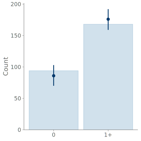
Bar graphs
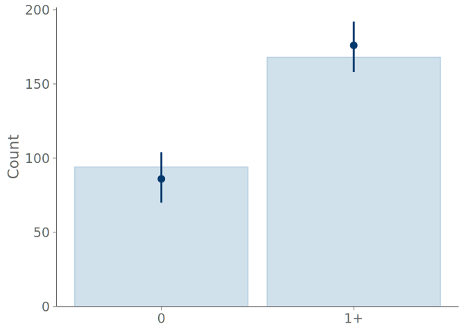
A bar graph consists of bars representing the frequencies of the observed values, and point intervals of the predictive means and central quantiles. These elements are positioned over each state of the observation distribution. Bar graphs are a common choice when summarizing discrete binary, categorical, or ordinal data and predictions. Although bar graphs can work well for predictive checking as part of rootgrams for count data, they are less useful when there are a small number of discrete values. In the extreme case of binary data, even a model with one parameter corresponding to the proportion of one class, can perfectly model the proportion, and the overlaid posterior predictive checking bar plots are useless (and KDE plots are even worse with misleading smoothing). Additionally, as shown in Figure 21 and Figure 22 below, any assessment that is more advanced than inspecting the relative frequencies of the discrete states, is impossible with the bar graphs. For example, under- and overconfidence, and symmetric confusion between states, is not visible in a graph.
Figure 20 (a) shows bar graphs summarizing the predictions of the intercept-only and negative binomial models for predicting the binary outcome of observing one or more roaches. Both bar graphs show the model predictions agreeing with the observations, and no clear difference in the predictions of the models can be seen.

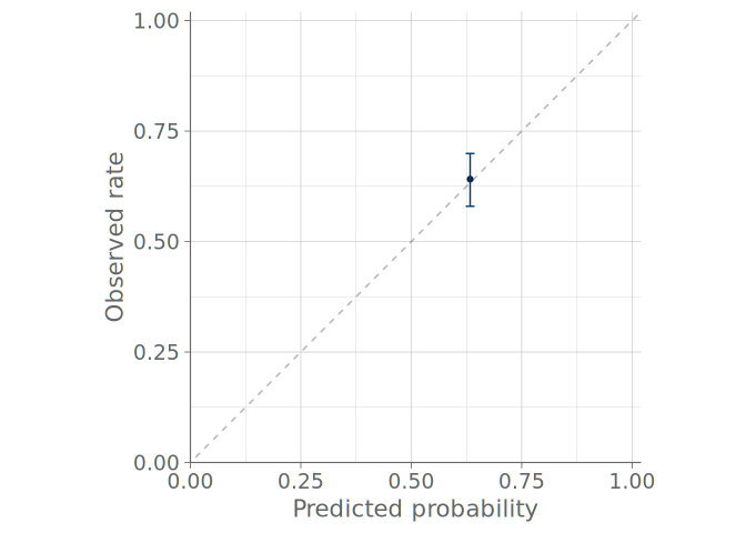
Binned calibration plots
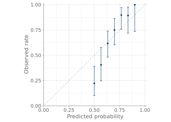
What could be argued to be the first step towards assessing calibration of the predictive probabilities in binary prediction tasks is the use of binned calibration plots (Niculescu-Mizil and Caruana 2005), also called calibration curves or reliability diagrams (DeGroot and Fienberg 1983). In these visualizations, the binary observations are divided into a predetermined number of uniform bins, based on the event probabilities predicted by the model. Comparing the mean predicted probability to the observed event rate within each bin allows assessing the calibration, or reliability, of the model. Typically, binned calibration plots include a binomial confidence intervals of the observed event rates. In practice, binned calibration plots suffer from similar drawbacks as histograms; the choice of binning is up to the user, and can cause the resulting plots to look drastically different, as shown by (Dimitriadis, Gneiting, and Jordan 2021).
Figure 20 (b) shows the binned calibration plots for the predictive distributions visualized previously through bar graphs. It is immediately clear that even though the probabilities predicted by the intercept-only model are calibrated, the model has no ability to discriminate between the cases where one is more or less likely to observe roaches. We can also see, that although the negative binomial model is better at discriminating the cases, it suffers from calibration issues and is especially under-confident at predicting cases where no roaches will be observed.
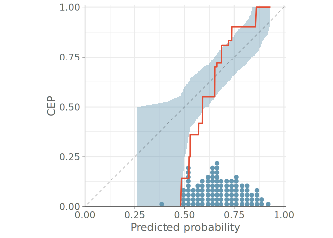
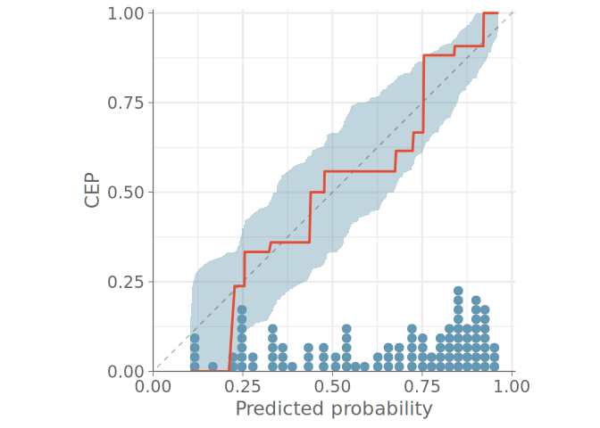
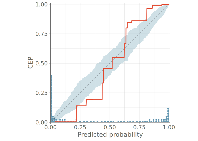
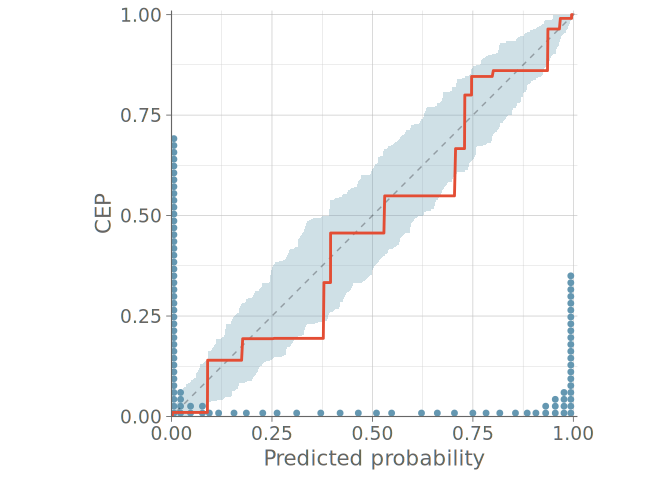
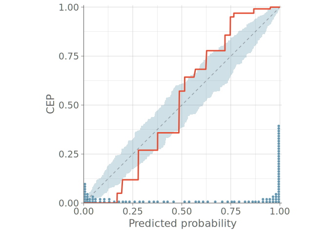
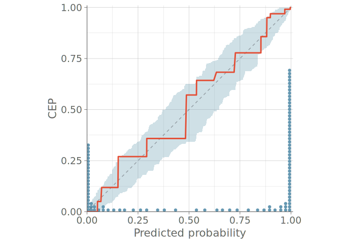
PAV-adjusted calibration plots
The ad-hoc binning decision has the potential to play a major role in the conclusions drawn from binned calibration plots. To address this, Dimitriadis, Gneiting, and Jordan (2021) propose a method where the observed binary events are replaced with conditional event probabilities (CEP), that is the probability that a certain event occurs given that the classifier has assigned a specific predicted probability. To compute the CEPs, the authors use the pool adjacent violators (PAV) algorithm (Ayer et al. 1955), which provides a non-parametric maximum likelihood solution to the problem of assigning CEPs that are monotonic with respect to the model predictions. This monotonicity assumption is reasonable for calibrated models, where higher predicted probabilities should correspond to higher actual event probabilities.
To aid in the calibration assessment, we employ the point-wise consistency bands introduced by (Dimitriadis, Gneiting, and Jordan 2021). These intervals show, how much variation should be expected from the calibration plot even if the model was perfectly calibrated.
Figure 20 (c) shows this PAV-adjusted calibration plot with 95% point-wise consistency bands computed from the posterior predictive distribution. First, we compute the CEPs using the posterior predictive means for each observation. Then we form the consistency bands by using the corresponding posterior predictive draws to determine the 95% credible intervals for CEPs of draws from the predictive distribution.
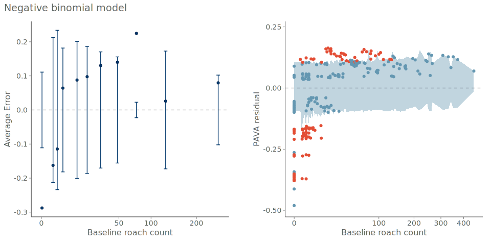
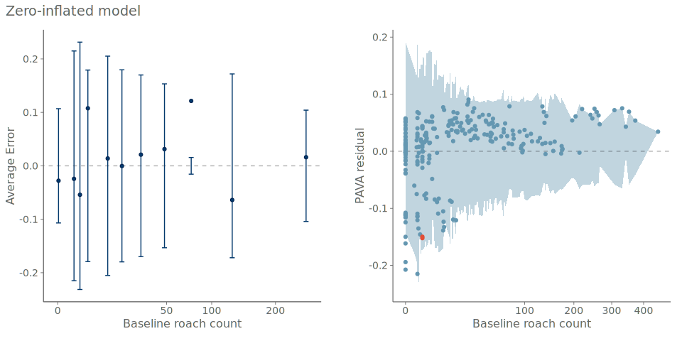
Residual plots
While binned and PAV-adjusted calibration plots are useful for assessing the overall predictive calibration of a model, the behavior conditional on individual predictors is often of interest to practitioners.
Residual plots are commonly deployed for assessing the deviation between observations and predictions (Gelman, Hill, and Vehtari 2020; Gelman et al. 2013; Agresti 2013). As with binned calibration plots, binning is used for transforming discrete outcomes into relative event frequencies.
Again, the ad-hoc choice of binning may result in vastly different plots, and thus we propose the use of PAV-adjusted CEPs, computed with regards to the predicted probabilities, in place of the discrete observations. Figure 24 shows an example of a PAV-adjusted residual plot for the roaches example.
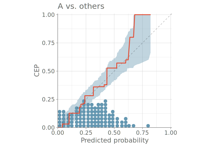
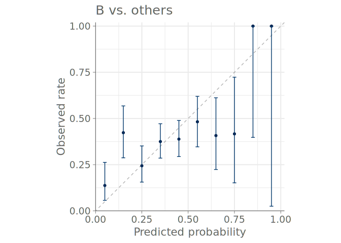
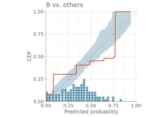
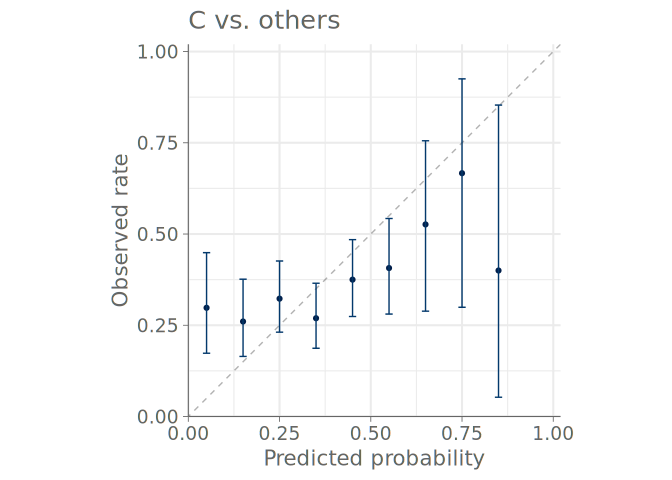
5 Visual predictive checks for categorical data
When the number of categories is relatively low, the methods presented for the binary case in Section 4 extend to the categorical case. In the same way as for binary data, even the simplest model is likely to have such parameters that the predictive probabilities match the observed frequencies and bar plots are useless. However, we can use the calibration of the binomial one-versus-others (OVO) distributions for each of the categorical cases. With a large number of categories, investigating one plot for each OVO calibration can be unwieldy, but scalar summaries of miscalibration for each category could be used to filter the set of individual cases before graphical inspection.
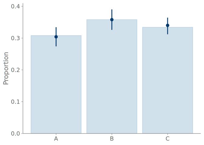
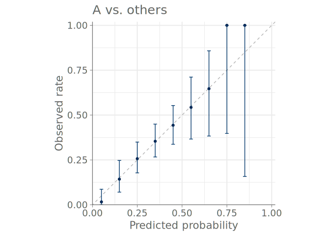
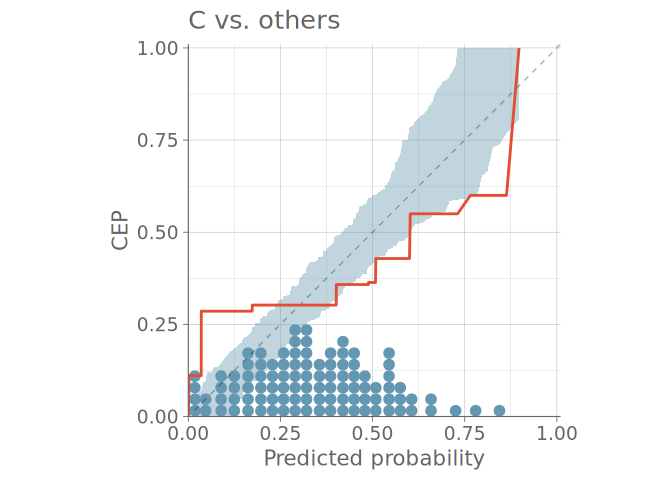
Figure 25 shows a predictive check using bar graphs for a predictive model with three distinct categories. Figure 26 shows both binned and PAV-adjusted calibration plots for the same model. No immediate calibration issues are visible for the model when predicting category A, but one can also see that cases, where the model would estimate the probability of any single category to be larger than 0.7 are rare – only one to three quantile dots are at values larger than 0.7. Additionally, both plots types show that the model confuses classes B and C, and is over confident in its predictions concerning these classes.
6 Visual predictive checks for ordinal data
Models for ordinal data often have such parameters that even the simplest model predictive probabilities match the observed frequencies and bar plots are useless (KDE plots are even worse with misleading smoothing). In the case of ordinal predictions, instead of looking at the OVO distributions, we can assess the calibration of the cumulative conditional event probabilities. This allows us to again use the toolset presented for binomial predictive checks in Section 4, now resulting in M-1 plots, where M is the number of possible distinct discrete cases.
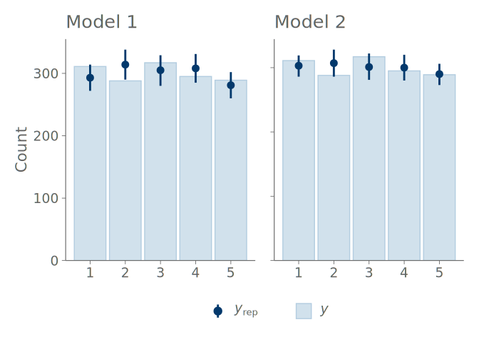
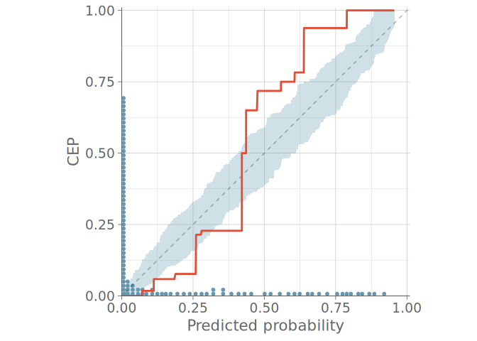
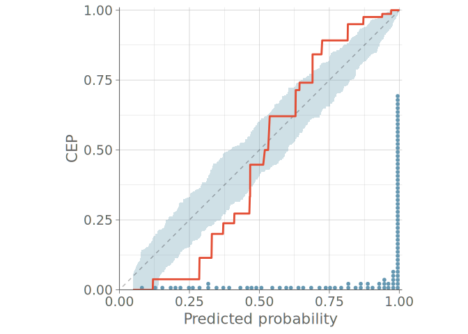
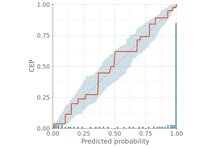
Figure 28 shows a PPC using bar graphs for two models without any sign of calibration issues in either predictive distribution. Figure 29 shows the PAV-adjusted calibration plots for each cumulative event probability. The diagrams for model 1 on the left show a calibration issue, with the calibration curves exhibiting an S-shape, indicative of under confidence in predicted probabilities.

7 Discussion
In this paper we discussed the current options for graphical predictive checking in Bayesian model checking workflows. As discussed, the type of data being modelled, and the type of model being applied are key considerations when choosing a particular approach. We strongly recommend that practitioners carefully consider the underlying assumptions being made by a chosen visualization and perform some form of diagnostic-check, such as the discussed PIT-ECDF, if unsure.
To summaries our recommendations, KDE plots are primarily only recommended for when a modeller is confident that the distribution is smooth (no point-masses or steps), or if there are many unique discrete values. If a KDE plot is going to be used for a bounded distribution, boundary corrections methods should be used, and we still recommend goodness-of-fit checking. Failing this, if the distribution has a continuous component, we recommend a quantile dot plot. For count distributions, we recommend a modified rootogram, plotting points and credible intervals instead of smoothed limits. For unordered discrete data, we recommend using a PAV-adjusted One-Versus-Others calibration plot. Finally, for ordered discrete data, we also recommend a PAV-adjusted calibration, but evaluating the cumulative conditional event probabilities.
It must be emphasized that these are only general recommendations. As we have presented above, these recommended plots may still fail to identify miscalibration or other goodness-of-fit issues in some situations. Careful consideration of model assumptions and application of diagnostics should always form part of the modeller’s standard practice. Many of our recommendations can be taken into account in the visual predictive checking software, for example, by giving a warning if a user tries to use overlaid KDE plot or bar plot for checking a model in case of binary data.
Acknowledgements
We acknowledge the support by the Research Council of Finland Flagship programme: Finnish Center for Artificial Intelligence and Research Council of Finland project (340721).
We would also like to thank the maintainers and contributors of the Open Source software used in creating the visualizations and examples presented in this article: R Core Team (2021); Wickham (2016), Kay (2023, 2024), Gabry et al. (2019) and Gabry and Mahr (2024) for their excellent visualization packages; Narasimhan et al. (2024) for implementation of the numerical integration used in the PIT computations for KDE densities; Turner (2023), Kuhn and Max (2008), and Dimitriadis, Gneiting, and Jordan (2021) for implementing functions used in making calibration plots; and Bürkner (2017, 2018, 2021), Gabry et al. (2024), Goodrich et al. (2024), and Team (2018) for developing the probabilistic programming software used in this article.
References
Research materials
Source files of this article, as well as supplementary materials providing additional detail into the examples and case-studies shown in this article, can be found at https://teemusailynoja.github.io/visual-predictive-checks. The version of the implementations used in this article can be found in Zenodo.
License
This work is licensed under a Creative Commons Attribution 4.0 International License.
Conflicts of interest
The authors declare that there are no competing interests.