The illusory promise of the Aligned Rank Transform

A systematic study of rank transformations

Authors

Affiliations

Theophanis Tsandilas

Université Paris-Saclay, CNRS, Inria, LISN

Géry Casiez

Univ. Lille, CNRS, Inria, Centrale Lille, UMR 9189 CRIStAL

Under Review

This paper is under review on the experimental track of the Journal of Visualization and Interaction. See the reviewing process.

Abstract

Introduction

The Aligned Rank Transform (ART) is a popular statistical method, commonly used when the assumptions of parametric procedures, such as normality assumptions, are not met. Its popularity stems from several Monte Carlo experiments demonstrating that the method is robust and powerful. However, contrary experimental findings suggest that ART may be less robust compared to simpler rank transformation methods, failing to adequately control Type I error rates across various scenarios, including discrete data, skewed distributions, and distributions with unequal variances. These results have not gained attention within the Human-Computer Interaction community, where ART is routinely used.

Objectives

This research aims to clarify the contradictory findings from previous studies by reevaluating the robustness and effectiveness of ART. Its complementary goal is to investigate the performance of alternative nonparametric methods.

Methods

We conducted an extensive series of Monte Carlo experiments to systematically evaluate ART across a broad range of data distributions and experimental designs. Our comparative analysis includes two alternative transformation methods: the simple rank transformation and the inverse normal transformation, along with parametric ANOVA without transformation. Additionally, we present supplementary experiments involving other competitive nonparametric methods in the appendix.

Our experimental method is based on generalized linear models and latent variable modeling, enabling precise control over main and interaction effects across diverse distributions. Throughout our analysis, we carefully address interpretation issues arising from the definition of the null hypothesis in nonlinear models. In addition to the experiments, we explore the behavior of ART through illustrative examples and reanalyze datasets from previously published user studies.

Results

Our results show that ART fails under a range of discrete distributions, including binomial data and Likert-type data with 5, 7, and 11 ordinal levels. Moreover, ART systematically confounds effects in skewed distributions or distributions with unequal variances. We report results for various experimental designs, including between-subject, within-subject, and mixed designs with two or three factors.

Surprisingly, ART functions as intended only under the strict assumption of a linear model with continuous responses, equal variances, and no missing data. In all other scenarios, it performs worse than simpler rank transformation methods and, in many cases — such as with ordinal data — significantly worse than parametric ANOVA. Our analysis of real-world data further demonstrates that using ART often leads to incorrect conclusions. By contrast, the inverse normal transformation proves to be the most robust nonparametric method, though we also identify scenarios where it inflates errors and distorts effects.

In addition, our results show that testing interactions in the presence of multiple main effects remains a challenge for all methods. We raise awareness about previous warnings regarding the interpretation of removable interactions.

Conclusion

We conclude that ART is a flawed statistical method and should no longer be used. We recommend prioritizing parametric modeling approaches, including linear models and their generalizations. While we propose the inverse normal transformation as a generic nonparametric alternative, we caution researchers about the limitations and potential risks of rank-based procedures.

Materials

We provide supplementary materials with experimental code, raw experimental results, and detailed analyses of examples and case studies presented throughout the article. Source files of our article, appendix, and supplementary materials can also be found on OSF at https://osf.io/hs7j8.

Materials, Authorship, License, Conflicts

Research materials

We provide supplementary materials with experimental code, raw experimental results, and detailed analyses of examples and case studies presented throughout the article. Source files of our article, appendix, and supplementary materials can also be found on OSF at https://osf.io/hs7j8.

Authorship

Theophanis Tsandilas: Conceptualization, Methodology, Resources, Software, Formal Analysis, Investigation, Validation, Data Curation, Vizualization, Writing - Original Draft, Writing - Review & Editing. Géry Casiez: Conceptualization, Investigation, Writing - Review & Editing.

License

This work is licensed under a Creative Commons Attribution 4.0 International License.

Conflicts of interest

The authors declare that there are no competing interests.

1 Introduction

In Human-Computer Interaction (HCI) and many areas of the behavioral sciences, researchers frequently collect data through user studies. Such data are often messy, involve small sample sizes, and violate common statistical assumptions, such as the normality assumption. To address these challenges, researchers commonly rely on nonparametric tests, which require fewer assumptions about the underlying data. However, while nonparametric tests for simple one-factorial designs are well-established, researchers face challenges in selecting appropriate methods when dealing with multifactorial designs that require testing for both main effects and interactions.

The Aligned Rank Transform or ART (Higgins, Blair, and Tashtoush 1990; Salter and Fawcett 1993; Wobbrock et al. 2011) was introduced to address this problem by bridging the gap between nonparametric tests and ANOVA. Its popularity in HCI research has surged, in part due to the ARTool toolkit (Wobbrock et al. 2011; Kay et al. 2021), which makes the method easy to apply. Oppenlaender and Hosio (2025) identify the paper by Wobbrock et al. (2011) as a major milestone in HCI research, ranking it third in terms of citations in the ACM CHI Proceedings (1981-2024), behind Braun and Clark’s (2006) article on thematic analysis and Hart and Staveland’s (1988) work on the NASA-TXL index.

However, given their substantial impact on research outcomes in our community, these widely adopted methods deserve closer scrutiny. As the first author previously argued (Tsandilas 2018), the HCI community lacks sufficiently expertise to critically assess the validity of statistical techniques. Our findings suggest that the widespread use of ART largely stems from limited awareness of its underlying assumptions. Many researchers treat ART as a general-purpose nonparametric alternative when ANOVA’s assumptions are violated, overlooking the fact that ART’s alignment mechanism imposes even stricter assumptions — including linear relationships between the predictors and responses, equal variances, and continuous data.

Early Monte Carlo experiments in the 1990s (Salter and Fawcett 1993; Mansouri and Chang 1995) and more recent studies (Elkin et al. 2021) suggested that ART is a robust alternative to ANOVA when normality assumptions are violated. These results have contributed to ART’s reputation as a well-established method. However, other research (Lüpsen 2017, 2018) raised concerns about the robustness of the method, demonstrating that ART fails to control the Type I error rate in many scenarios, such as when data are ordinal or are drawn from skewed distributions. Unfortunately, these warnings have received little attention, and many authors continue to rely on Wobbrock et al.’s (2011) assertion that “The ART is for use in circumstances similar to the parametric ANOVA, except that the response variable may be continuous or ordinal, and is not required to be normally distributed.”

This paper aims to clarify the severity of these issues and understand the potential risks of the method. We present the results of a series of Monte Carlo experiments in which we simulate a broad spectrum of distributions, both discrete and continuous. Throughout the analysis, we pay particular attention to how the definition of the null hypothesis affects the interpretation of results. To improve clarity and reproducibility, we decompose the study into multiple focused experiments, each targeting a specific factor (e.g., sample size, experimental design, standard-deviation ratio) or outcome measure (Type I error rate, statistical power, and the precision of effect size estimates).

Our findings corroborate Lüpsen’s alarming conclusions. We provide overwhelming evidence that ART confounds effects and raises Type I error rates at very high levels across a wide range of non-normal distributions, including skewed, binomial, and ordinal distributions, as well as distributions with unequal variances. These issues persist for both main and interaction effects. Our results further show that simpler rank transformation methods outperform ART, while parametric ANOVA generally poses fewer risks than ART when distributions deviate from normal. Based on these results, we conclude that ART is not a viable analysis method and should be abandoned. We offer recommendations for alternative analysis methods, while we also raise warnings about the analysis and interpretation of interaction effects.

Illustrative example

We will begin with an illustrative example to demonstrate how the aligned rank transform can lead to an increase in false positives and a significant inflation of observed effects. This example will also serve as a brief introduction to the key concepts and methods employed throughout the paper.

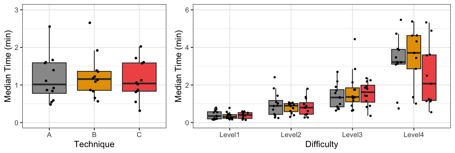
Suppose a team of HCI researchers conduct an experiment to compare the performance of three user interface techniques (A, B, and C) that help users complete image editing tasks of four different difficulty levels. The experiment follows a fully balanced \(4 \times 3\) within-subject factorial design, where each participant (N = 12) performs 12 tasks in a unique order. The researchers measure the time that it takes participants to complete each task. In addition, the participants rate their perceived efficiency completing each task, using an ordinal scale with five levels: (1) inefficient, (2) somewhat inefficient, (3) neutral, (4) somewhat efficient, and (5) efficient.

The following table presents the experimental results:

Example dataset: Time (in minutes) spent by 12 participants and their perceived efficiency (ordinal scale) for four difficulty levels and three user interface techniques. Scroll down for full results.

Participant	Difficulty	Technique	Time	Perceived_Efficiency
P01	Level1	A	0.20	efficient
P01	Level1	B	0.17	somewhat efficient
P01	Level1	C	0.14	neutral
P01	Level2	A	0.45	efficient
P01	Level2	B	0.50	efficient
P01	Level2	C	0.27	neutral
P01	Level3	A	0.64	efficient
P01	Level3	B	0.63	efficient
P01	Level3	C	0.83	somewhat efficient
P01	Level4	A	0.75	efficient
P01	Level4	B	1.35	neutral
P01	Level4	C	1.25	somewhat efficient
P02	Level1	A	0.71	efficient
P02	Level1	B	0.47	efficient
P02	Level1	C	0.59	efficient
P02	Level2	A	1.82	efficient
P02	Level2	B	0.87	efficient
P02	Level2	C	1.29	efficient
P02	Level3	A	1.35	efficient
P02	Level3	B	4.44	efficient
P02	Level3	C	1.92	efficient
P02	Level4	A	3.22	efficient
P02	Level4	B	9.62	efficient
P02	Level4	C	5.33	efficient
P03	Level1	A	0.55	efficient
P03	Level1	B	0.21	efficient
P03	Level1	C	0.43	efficient
P03	Level2	A	0.88	efficient
P03	Level2	B	1.07	efficient
P03	Level2	C	1.36	efficient
P03	Level3	A	0.85	efficient
P03	Level3	B	0.66	efficient
P03	Level3	C	2.19	efficient
P03	Level4	A	3.21	efficient
P03	Level4	B	3.44	efficient
P03	Level4	C	2.07	efficient
P04	Level1	A	0.54	efficient
P04	Level1	B	0.41	efficient
P04	Level1	C	0.52	neutral
P04	Level2	A	1.02	somewhat efficient
P04	Level2	B	0.61	efficient
P04	Level2	C	0.80	efficient
P04	Level3	A	2.19	neutral
P04	Level3	B	1.75	efficient
P04	Level3	C	2.36	efficient
P04	Level4	A	9.82	efficient
P04	Level4	B	4.32	efficient
P04	Level4	C	3.58	efficient
P05	Level1	A	0.79	efficient
P05	Level1	B	0.78	efficient
P05	Level1	C	0.45	neutral
P05	Level2	A	2.41	efficient
P05	Level2	B	0.99	efficient
P05	Level2	C	1.80	efficient
P05	Level3	A	2.70	efficient
P05	Level3	B	2.85	efficient
P05	Level3	C	2.25	efficient
P05	Level4	A	3.13	efficient
P05	Level4	B	5.38	somewhat efficient
P05	Level4	C	6.24	efficient
P06	Level1	A	0.64	efficient
P06	Level1	B	0.23	efficient
P06	Level1	C	0.34	efficient
P06	Level2	A	0.90	efficient
P06	Level2	B	0.93	efficient
P06	Level2	C	0.45	efficient
P06	Level3	A	1.32	efficient
P06	Level3	B	1.34	efficient
P06	Level3	C	1.80	efficient
P06	Level4	A	5.47	efficient
P06	Level4	B	4.64	efficient
P06	Level4	C	2.50	efficient
P07	Level1	A	0.17	efficient
P07	Level1	B	0.17	efficient
P07	Level1	C	0.16	efficient
P07	Level2	A	0.24	efficient
P07	Level2	B	0.30	neutral
P07	Level2	C	0.27	efficient
P07	Level3	A	0.72	inefficient
P07	Level3	B	1.30	efficient
P07	Level3	C	0.36	efficient
P07	Level4	A	1.06	neutral
P07	Level4	B	1.01	efficient
P07	Level4	C	0.55	efficient
P08	Level1	A	0.36	efficient
P08	Level1	B	0.38	efficient
P08	Level1	C	0.22	efficient
P08	Level2	A	0.69	efficient
P08	Level2	B	1.02	efficient
P08	Level2	C	0.89	neutral
P08	Level3	A	0.99	efficient
P08	Level3	B	1.75	efficient
P08	Level3	C	1.15	efficient
P08	Level4	A	3.87	efficient
P08	Level4	B	4.63	efficient
P08	Level4	C	4.89	efficient
P09	Level1	A	0.33	efficient
P09	Level1	B	0.24	efficient
P09	Level1	C	0.21	efficient
P09	Level2	A	0.39	efficient
P09	Level2	B	1.01	efficient
P09	Level2	C	0.42	efficient
P09	Level3	A	0.79	efficient
P09	Level3	B	1.17	efficient
P09	Level3	C	1.86	efficient
P09	Level4	A	3.47	neutral
P09	Level4	B	2.86	efficient
P09	Level4	C	1.21	efficient
P10	Level1	A	0.18	efficient
P10	Level1	B	0.24	efficient
P10	Level1	C	0.59	neutral
P10	Level2	A	0.27	efficient
P10	Level2	B	0.77	neutral
P10	Level2	C	0.61	efficient
P10	Level3	A	1.57	efficient
P10	Level3	B	0.90	efficient
P10	Level3	C	1.43	somewhat efficient
P10	Level4	A	4.73	efficient
P10	Level4	B	3.71	efficient
P10	Level4	C	1.13	efficient
P11	Level1	A	0.15	somewhat efficient
P11	Level1	B	0.57	somewhat efficient
P11	Level1	C	0.38	somewhat inefficient
P11	Level2	A	1.43	neutral
P11	Level2	B	0.39	efficient
P11	Level2	C	0.79	efficient
P11	Level3	A	1.90	efficient
P11	Level3	B	2.14	neutral
P11	Level3	C	0.89	somewhat inefficient
P11	Level4	A	3.92	neutral
P11	Level4	B	7.19	somewhat efficient
P11	Level4	C	3.62	inefficient
P12	Level1	A	0.23	efficient
P12	Level1	B	0.41	efficient
P12	Level1	C	0.56	efficient
P12	Level2	A	1.09	efficient
P12	Level2	B	1.06	efficient
P12	Level2	C	0.98	efficient
P12	Level3	A	1.70	efficient
P12	Level3	B	1.39	efficient
P12	Level3	C	1.42	efficient
P12	Level4	A	3.09	efficient
P12	Level4	B	6.24	efficient
P12	Level4	C	1.14	efficient

The experiment is hypothetical but has similarities with real-world experiments, e.g., see the experiments of Fruchard et al. (2023).

Time performance. Time measurements have been randomly sampled from a population in which: (1) Difficulty has a large main effect; (2) Technique has no main effect; and (3) there is no interaction effect between the two factors. To generate time values, we drew samples from a log-normal distribution. The log-normal distribution is often a good fit for real-world measurements that are bounded by zero and have low means but large variance (Limpert, Stahel, and Abbt 2001). Task-completion times are good examples of such measurements (Sauro and Lewis 2010).

Figure 1 presents two boxplots that visually summarize the main effects observed through the experiment. We plot medians to account for the fact that distributions are skewed. We observe that differences in the overall time performance of the three techniques are not visually clear, although the overall median time is somewhat higher for Technique B. In contrast, time performance clearly deteriorates as task difficulty increases. We also observe that for the most difficult tasks (Level 4), the median time for Technique C is lower than the median time for Techniques A and B, so we may suspect that Difficulty interacts with Technique. However, since the spread of observed values is extremely large and the number of data points is small, such differences could result from random noise.

Figure 1: Boxplots summarizing time performance results for our illustrative example. Dots represent the median time for each individual participant.

We opt for a multiverse analysis (Dragicevic et al. 2019) to analyze the data, where we conduct a repeated-measures ANOVA with four different data-transformation methods:

1. Log transformation (LOG). Data are transformed with the logarithmic function. For our data, this is the most appropriate method as we drew samples from a log-normal distribution.

2. Aligned rank transformation (ART). Data are transformed and analyzed with the ARTool (Wobbrock et al. 2011; Elkin et al. 2021).

3. Pure rank transformation (RNK). Data are transformed with the original rank transformation (Conover and Iman 1981), which does not perform any data alignment.

4. Inverse normal transformation (INT). The data are transformed by using their normal scores. This rank-based method is simple to implement and has been commonly used in some disciplines. However, it has also received criticism (Beasley, Erickson, and Allison 2009).

For comparison, we also report the results of the regular parametric ANOVA with no transformation (PAR). To simplify our analysis and like Elkin et al. (2021), we consider random intercepts but no random slopes. For example, we use the following R code to create the model for the log-transformed response:

m.log <- aov(log(Time) ~ Difficulty*Technique + Error(Participant), data = df)

Alternatively, we can use a linear mixed-effects model, treating the participant identifier as a random effect:

m.log <- lmer(log(Time) ~ Difficulty*Technique + (1|Participant), data = df)

The table below presents the p-values for the main effects of the two factors and their interaction:

p-values for main and interaction effects

	PAR	LOG	ART	RNK	INT
Difficulty	\(1.8 \times 10^{-26}\)	\(8.1 \times 10^{-47}\)	\(9.0 \times 10^{-43}\)	\(4.3 \times 10^{-46}\)	\(4.4 \times 10^{-44}\)
Technique	\(.10\)	\(.18\)	\(.00062\)	\(.38\)	\(.17\)
Difficulty \(\times\) Technique	\(.056\)	\(.10\)	\(.0017\)	\(.24\)	\(.23\)

The disparity in findings between ART and the three alternative transformation methods is striking. ART suggests that three is strong statistical evidence for all three effects. What adds to the intrigue is the fact that ART’s p-values for Technique and its interaction with Difficulty are orders of magnitude lower than the p-values obtained from all other methods. We will observe similar discrepancies if we conduct contrast tests with the ART procedure (Elkin et al. 2021), though we leave this as an exercise for the reader.

We also examine effect size measures, which are commonly reported in scientific papers. The table below presents results for partial \(\eta^2\), which describes the ratio of variance explained by a variable or an interaction:

partial \(\eta^2\) and its 95% confidence interval

	PAR	LOG	ART	RNK	INT
Difficulty	\(.64\ [.55, 1.0]\)	\(.83\ [.79, 1.0]\)	\(.80\ [.76, 1.0]\)	\(.83\ [.79, 1.0]\)	\(.81\ [.77, 1.0]\)
Technique	\(.04\ [.00, 1.0]\)	\(.03\ [.00, 1.0]\)	\(.11\ [.03, 1.0]\)	\(.02\ [.00, 1.0]\)	\(.03\ [.00, 1.0]\)
Difficulty \(\times\) Technique	\(.10\ [.00, 1.0]\)	\(.08\ [.00, 1.0]\)	\(.16\ [.04, 1.0]\)	\(.06\ [.00, 1.0]\)	\(.06\ [.00, 1.0]\)

We observe that ART exaggerates both the effect of Technique and its interaction with Difficulty. This example demonstrates a more general problem with ART’s alignment mechanism under long-tailed distributions. ART tends to confound effects: a strong effect on a single factor often leads the method to detect spurious effects on other factors or to identify non-existent interactions.

Perceived efficiency. The perceived efficiency ratings were randomly sampled from a population with no main effect on any of the two factors and no interaction effect. Figure 2 shows that participants’ ratings are concentrated at the higher end of the scale but with no clear trends.

Figure 2: Boxplots summarizing the results on efficiency as perceived by participants. Circles represent the mean rating of each individual participant.

For our analysis, we compare the results of PAR, ART, RNK, and INT, since LOG is not relevant for this type of data. We also report the results of the Friedman test (Friedman 1940) for each factor, where we first aggregate the data by taking the mean over the other factor. Results are as follows:

p-values for main and interaction effects

	PAR	ART	RNK	INT	Friedman Test
Difficulty	\(.93\)	\(.0011\)	\(.86\)	\(.88\)	\(.83\)
Technique	\(.18\)	\(.00016\)	\(.32\)	\(.23\)	\(.24\)
Difficulty \(\times\) Technique	\(.27\)	\(.10\)	\(.33\)	\(.34\)

ART’s p-values for the two main effects are surprisingly low, while no other method shows any substantial evidence for such effects. We also present the methods’ effect size estimates:

partial \(\eta^2\) and its 95% confidence interval

	PAR	ART	RNK	INT
Difficulty	\(.004\ [.00, 1.0]\)	\(.12\ [.03, 1.0]\)	\(.006\ [.00, 1.0]\)	\(.005\ [.00, 1.0]\)
Technique	\(.03\ [.00, 1.0]\)	\(.13\ [.05, 1.0]\)	\(.02\ [.00, 1.0]\)	\(.02\ [.00, 1.0]\)
Difficulty \(\times\) Technique	\(.06\ [.00, 1.0]\)	\(.04\ [.00, 1.0]\)	\(.05\ [.00, 1.0]\)	\(.05\ [.00, 1.0]\)

The discrepancies between ART’s estimates for the two main effects and those of the other methods are large. As we demonstrate in this paper, such discrepancies stem from ART’s inability to handle discrete distributions. The issue becomes more pronounced with larger sample sizes. Lüpsen (2017) previously warned researchers about this problem, but his warnings have largely been ignored.

Overview

The above example does not reflect a rare phenomenon. We will show that ART’s error inflation is systematic for a range of distributions that deviate from normality, both continuous and discrete.

The paper is structured as follows. Section 2 introduces nonparametric tests and rank transformations, and explains how ART is constructed. It also provides a summary of previous experimental results regarding the robustness of ART and other related rank-based procedures, along with a survey of recent studies using ART. Section 3 clarifies the method’s distributional assumptions. Section 4 investigates issues regarding the definition of the null hypothesis and the interpretation of main and interaction effects. Section 5 outlines our experimental methodology, while Section 6 presents our findings. Section 7 revisits results of previous studies employing ART and illustrates how its application can lead to erroneous conclusions. Section 8 offers recommendations for researchers. Finally, Section 9 concludes the paper.

In addition to the main sections of the paper, we provide an appendix (see Appendix I) with results from additional Monte Carlo experiments.

2 Background

We provide background on the history, scope, construction, and use of rank transformation methods, with a particular focus on ART. Additionally, we summarize the results of previous evaluation studies and position our own work within this context.

Nonparametric statistical tests

Classical ANOVA and linear regression are based on a linear model in which the error terms (residuals) are assumed to be independent, homoscedastic, and normally distributed. When sample sizes are sufficiently large, violations of the normality assumption become less problematic for inference on model coefficients because, under fairly general conditions, the sampling distributions of these coefficients are approximately normal (Central Limit Theorem). As a result, ANOVA is often reasonably robust to moderate departures from normality. However, this robustness weakens with small sample sizes, strong skewness, heavy tails, outliers, or heteroscedasticity, all of which can substantially affect Type I error rates and power.

The goal of nonparametric procedures is to mitigate these problems by making fewer and weaker assumptions about the underlying distributions. The original idea of replacing the data values by their ranks goes back to Spearman (1904). The key advantage of ranks is that they preserve the monotonic relationship of values while also allowing the derivation of an exact probability distribution. This probability distribution can then be used for statistical inference, such as calculating a p-value. The idea of using ranks was adopted by other researchers, leading to the development of various nonparametric tests commonly used today. Representative examples include the Mann-Whitney U test (Mann and Whitney 1947) and the Kruskal–Wallis test (Kruskal and Wallis 1952) for independent samples, and the Wilcoxon sign-rank test (Wilcoxon 1945) and the Friedman test (Friedman 1940) for paired samples and repeated measures.

Rank transformations

The scope of classical nonparametric tests is limited, as they only support simple experimental designs with a single independent variable. Rank transformations aim to address this limitation by bridging the gap between nonparametric statistics and ANOVA.

The rank transform. Conover (2012) provides a comprehensive introduction to the simple rank transform, which consists of sorting the raw observations and replacing them by their ranks. In the presence of ties, tied observations are assigned fractional ranks equal to their average order position in the ascending sequence of values. For example, the two \(0.3\) instances of the \(Y\) responses in Figure 3 (a), which are the smallest values in the dataset, receive a rank of \(1.5\) (see \(rank(Y)\)), while the next value (a \(0.4\)) in the sequence receives a rank of \(3\).

Conover and Iman (1981) showed that, for one-factor designs, applying ANOVA to these ranks yields tests that are asymptotically equivalent or good replacements of traditional nonparametric tests (see Section 4). However, a series of studies in the 80s raised caution flags on the use of the method, showing that it may confound main and interaction effects in two-factor and three-factor experimental designs. For an extensive review of these studies, we refer readers to Sawilowsky (1990).

The aligned rank transform. In response to these negative findings, researchers turned to aligned (or adjusted) rank transformations. Sawilowsky (1990) reviews several variants of aligned rank-based transformations (ART) and tests, while Higgins, Blair, and Tashtoush (1990) describe the specific ART method that we evaluate in this paper for two-factor designs. Wobbrock et al. (2011) later generalized the method to more than two factors, and more recently, Elkin et al. (2021) extended it to multifactor contrast testing.

Figure 3 explains the general method for a design with two factors, \(A\) and \(B\). The key intuition behind the transform is that responses are ranked after they are aligned, such that effects of interest are separated from other effects. This implies that for each effect, either main or interaction, a separate ranking is produced. This is clearly illustrated in the example dataset shown in Figure 3 (a), where each aligned ranking (\(ART_A\), \(ART_B\), and \(ART_{AB}\)) is for testing a different effect (\(A\), \(B\), and \(A \times B\), respectively).

Figure 3: Example showing the use of the rank, ART, and INT transformation methods (a). Construction of ART for a two-factor design (b,c), where \(Y_{ijk}\) represents the response of the \(k^{th}\) subject for \(A=a_i\) and \(B=b_j\).

Figure 3 (b-c) details the calculation of the transformation, where we highlight the following terms: (i) residuals (in yellow) that represent the unexplained error (due to individual differences in our example); (ii) main effects (in green and pink) estimated from the observed means of the individual levels of the two factors; and (iii) interaction effect estimates (in blue). Observe that the estimates of the two main effects are subtracted from the interaction term. The objective of this approach is to eliminate the influence of main effects when estimating interaction effects.

Notice that even in this very small dataset (\(n = 2\)), the three ART rankings are distinct from one another and also differ significantly from the ranking produced by a simple rank transformation. Interestingly, identical responses (e.g., the two values of \(0.3\)) can be assigned very different ranks, while responses that differ substantially (e.g., \(0.3\) and \(3.0\)) may receive the same rank. More surprisingly, larger values can receive lower ranks — revealing that ART is a non-monotonic transformation. For instance, for subject \(s_1\) under condition \(b_1\), the responses are \(0.4\) and \(0.8\) for \(a_1\) and \(a_2\), yet their respective \(ART_A\) ranks are \(7.5\) and \(3.0\). In this case, ART significantly distorts the actual difference between the two groups, \(a_1\) and \(a_2\).

As we will show later, this behavior can lead to unstable results and misleading conclusions, and it represents a central flaw of the method. For example, running a repeated-measures ANOVA on these ART ranks yields a p-value of \(.044\) for the effect of \(A\). In contrast, using a repeated-measures ANOVA on the ranks of simple rank transformation produces a p-value of \(.46\), while applying a log-transformation — more appropriate for this type of data — yields a p-value of \(.85\).

This is not the only alignment technique discussed in the literature. Sawilowsky (1990) suggests that, at least for balanced designs, interactions could also be removed when aligning main effects, in the same way main effects are removed when aligning interactions. This approach is also taken by Leys and Schumann (2010), who derived a common ranking for both main effects after subtracting the interaction term. We do not evaluate these alternative alignment methods in this paper, as they are, to the best of our knowledge, not commonly used in practice.

The inverse normal transform. A third transformation method we evaluate is the rank-based inverse normal transformation (INT). INT has been in use for over 70 years (Waerden 1952) and exists in several variations (Beasley, Erickson, and Allison 2009; Solomon and Sawilowsky 2009). Its general formulation is as follows:

\[ INT(Y) = \Phi^{-1}(\frac{rank(Y) - c}{N - 2c + 1}) \tag{1}\]

where \(N\) is the total number of observations and \(\Phi^{-1}\) is the standard normal quantile function, which transforms a uniform distribution of ranks into a normal distribution. Different authors have used a different parameter \(c\). In our experiments, we use the Rankit formulation (Bliss, Greenwood, and White 1956), where \(c = 0.5\), since past simulation studies (Solomon and Sawilowsky 2009) have shown that it is more accurate than alternative formulations. However, as Beasley, Erickson, and Allison (2009) report, the choice of \(c\) is of minor importance. For our experiments, we implement the INT method in R as follows:

INT <- function(x){
    qnorm((rank(x) - 0.5)/length(x))
}

Figure 3 (a) shows how this function transforms the responses for our example dataset.

Other non-parametric rank-based methods. Several other rank-based statistical tests handle interactions, with the ANOVA-type statistic (ATS) (Brunner and Puri 2001) being the most representative one. Kaptein, Nass, and Markopoulos (2010) introduced this method to the HCI community, advocating its use for analyzing Likert-type data as an alternative to parametric ANOVA. Beyond ATS, Lüpsen (2017, 2018, 2023) examined several other multifactorial nonparametric methods. In particular, the author evaluated the hybrid ART+INT technique proposed by Mansouri and Chang (1995), which applies INT on the ranks of ART. He also tested multifactorial generalizations of the van der Waerden test (Waerden 1952) and the Kruskal-Wallis and Friedman tests (Kruskal and Wallis 1952; Friedman 1940). The former is based on INT, but instead of using F-tests on the transformed values as part of ANOVA, it computes \(\chi^2\) ratios over sums of squares. These two methods are not widely available, but R implementations can be obtained from Lüpsen’s website (Lüpsen 2021).

Experimental evaluations

Previous studies have evaluated ART and related procedures using various Monte Carlo simulations, often producing conflicting results and conclusions.

Results in support of ART. A number of experiments conducted during the 80s and 90s suggested that ART is robust for testing interaction effects. Noteworthy instances include studies, such as those by Salter and Fawcett (1993), which compared the method to parametric ANOVA. The authors found that ART remains robust even in the presence of outliers or specific non-normal distributions, such as the logistic, exponential, and double exponential distributions. Their findings indicated only a marginal increase in error rates (ranging from 6.0% to 6.3% instead of the expected 5%) when applied to the exponential distribution. Furthermore, ART demonstrated superior statistical power compared to parametric ANOVA. Mansouri and Chang (1995) evaluated ART under a different set of non-normal distributions (normal, uniform, log-normal, exponential, double exponential, and Cauchy) in the presence of increasing main effects. Except for the Cauchy distribution, ART maintained Type I error rates close to nominal levels across all scenarios, irrespective of the magnitude of main effects. In contrast, the error rates of the rank transformation reached very high levels (up to \(100\%\)) as the magnitude of main effects increased, even under the normal distribution. ART only failed under the Cauchy distribution, which is well-known to be pathological.

More recently, Elkin et al. (2021) compared ART to parametric t-tests for testing multifactor contrasts under six distributions: normal, log-normal, exponential, double exponential, Cauchy, and Student’s t-distribution (\(\nu=3\)). Their results confirmed that ART keeps Type I error rates close to nominal levels across all distributions, except for the Cauchy distribution. In addition, they found that ART exhibits a higher power than the t-test.

While most evaluation studies have focused on continuous distributions, Payton et al. (2006) have also studied how various transformations (rank, ART, log-transform, and squared-root transform) perform under the Poisson distribution, focusing again on interaction effects when main effects were present. The authors found that ART and parametric ANOVA (no transformation) performed best, keeping Type I error rates close to nominal levels. All other transformations inflated error rates.

Warnings. While the above results indicate that ART is a robust method, other studies have identified some serious issues. The second author of this paper has observed that, in certain cases, ART seems to detect spurious effects that alternative methods fail to identify (Casiez 2022). Such informal observations, conducted with both simulated and real datasets, motivated us to delve deeper into the existing literature.

Carletti and Claustriaux (2005) report that “aligned rank transform methods are more affected by unequal variances than analysis of variance especially when sample sizes are large.” Years later, Lüpsen (2018) conducted a series of Monte Carlo experiments, comparing a range of rank-based transformations, including the rank transformation, ART, INT, a combination of ART and INT (ART+INT), and ATS. His experiments focused on a \(2 \times 4\) balanced between-subject design and a \(4 \times 5\) severely unbalanced design and tested normal, uniform, discrete uniform (integer responses from 1 to 5), log-normal, and exponential distributions, with equal or unequal variances. Furthermore, they tested both interaction and main effects when the magnitude of other effects increased. The results revealed that ART inflates error rates beyond acceptable levels in several configurations: right-skewed distributions (log-normal and exponential), discrete responses, unequal variances, and unbalanced designs. Lüpsen (2018) also found that using INT in combination with ART (ART+INT) is preferable to the pure ART technique. However, as the method still severely inflated error rates in many settings, Lüpsen (2018) concluded that both ART and ART+INT are “not recommendable.”

Another notable finding by Lüpsen (2018) was that the simple rank transformation “appeared not as bad as it is often described” (Lüpsen 2018), outperforming ART in many scenarios, such as discrete and skewed distributions, or distributions with unequal variances. These results are in full contradiction with the findings of Mansouri and Chang (1995).

The same author conducted an additional series of experiments (Lüpsen 2017), focusing on two discrete distributions (uniform and exponential) with a varying number of discrete levels: 2, 4, and 7 levels with integer values for the uniform distribution, and 5, 10, and 18 levels with integer values for the exponential distribution. Again, the Type I error rates of both ART and ART+INT reached very high levels, but error rates were especially pronounced when the number of discrete levels became small and the sample size increased. Given these results, the author’s conclusion was the following:

“the ART as well as the ART+INT cannot be applied to Likert and similar metric or ordinal scaled variables, e.g. frequencies like the number of children in a family or the number of goals, or ordinal scales with ranges from 1 to 5” (Lüpsen 2017).

Results on other rank-based methods. We are also interested in understanding how ART compares with INT, which is frequently used in some research domains, such as genetics research (Beasley, Erickson, and Allison 2009). Beasley, Erickson, and Allison (2009) conducted an extensive evaluation of the method and reached the conclusion that “INTs do not necessarily maintain proper control over Type 1 error rates relative to the use of untransformed data unless they are coupled with permutation testing.” Lüpsen (2018) included INT in his evaluation and found that in most cases, it maintained better control of Type I error rates compared to ART and the pure rank transformation, while also presenting a higher statistical power. However, he also identified several cases where INT failed to sufficiently control for Type I errors, such as design configurations with unequal variances in unbalanced designs or skewed distributions, and when testing interactions in the presence of non-null main effects.

In addition to INT, Lüpsen (2018) evaluated the ATS method but found it to suffer from low power while presenting similar challenges as the rank transformation with regard to Type I error rates. Amongst all evaluated methods, the author identified the generalized van der Waerden test as the method that provided the best overall control of Type I error rates. More recently, Lüpsen (2023) conducted a new series of experiments testing rank-based nonparametric methods on split-plot designs with two factors. While the author reported on various tradeoffs of the methods, he concluded that overall, the generalized van der Waerden test and the generalized Kruskal-Wallis and Friedman tests were the best performing methods.

The use of ART in experimental research

To get a sense of how frequently ART is used in experimental research, we examined the citations of ARTool (Wobbrock et al. 2011) indexed by Google Scholar. As shown in Figure 4), the rate of citations to the original CHI 2011 paper introducing the method to the HCI community is steadily increasing, with over 400 citations in 2023 alone.

Figure 4: Citations of the CHI 2011 paper on ARTool (Wobbrock et al. 2011) as shown in Google Scholar on 28 April 2024. We analyzed the 439 citing bibliographic entries of 2023 in more detail. Note: Citations have continued to increase throughout the 2024–2025 period, and Google Scholar identifies about 680 citations in 2025 alone.

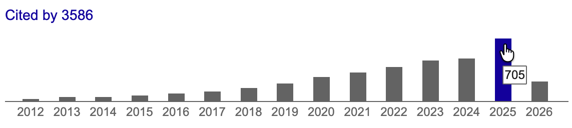
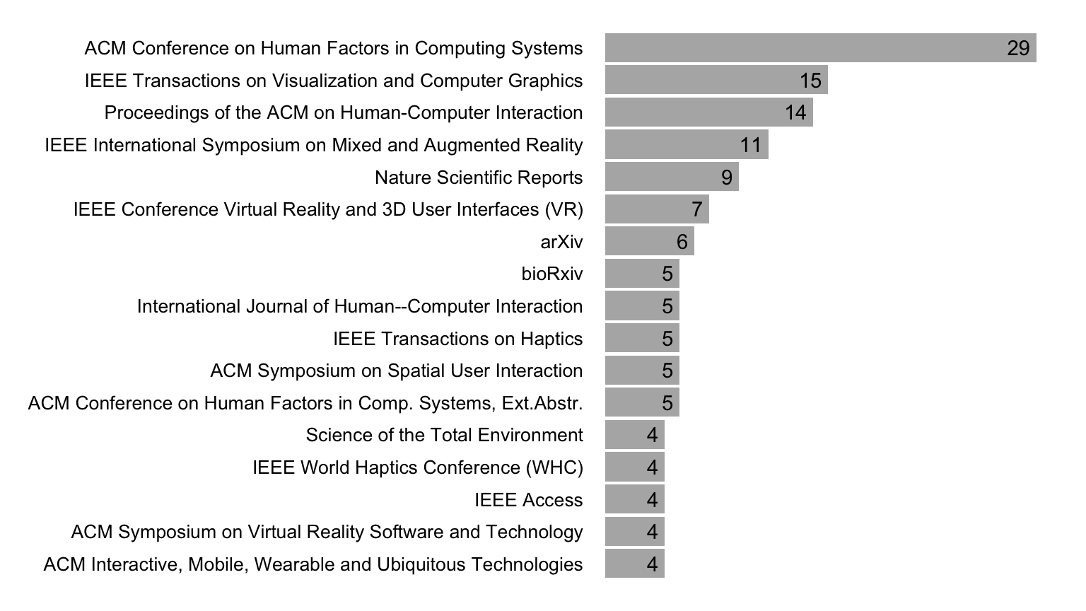
Figure 5 presents the most frequently citing venues for 2023. We observe that the HCI, Augmented Reality (AR), and Virtual Reality (VR) venues dominate these citations. However, we found that ARTool is used in other scientific disciplines. For example, among the papers published in 2023, we counted nine Nature Scientific Reports and a total of 25 articles appearing in journals with the words “neuro” or “brain” in their title, including the Journal of Neuropsychology (three citations), the Journal of Neuroscience (two citations), the Journal of Cognitive Neuroscience (two citations), Neuropsychologia (two citations), Nature Neuroscience, Neuropharmacology, Brain, and NeuroImage.

Figure 5: Publication venues with the highest number of citations to ARTool (Wobbrock et al. 2011) in 2023. Note that among the articles published in the IEEE Transactions on Visualization and Computer Graphics, eight articles appeared at the IEEE International Symposium on Mixed and Augmented Reality (IEEE ISMAR’23), and three articles appeared at the IEEE Conference on Virtual Reality and 3D User Interfaces (IEEE VR’23). So the total number of citing articles appearing at these two venues is 19 for IEEE ISMAR’23 and 10 for IEEE VR’23.

To gain insights into the prevalent experimental designs using ART, we examined a subset of citing papers comprising the 39 most recent English publications as of November 2023. Among these, 25 report using a within-subject design, three papers report using a between-subject design, while 11 papers report using a mixed design that involved both between- and within-subject factors. The number of factors ranges from one to five, with two factors representing approximately 64% of the experimental designs. Participant counts in these studies vary between 12 and 468, with a median of 24 participants. Within-cell sample sizes (n) range from 8 to 48, with a median of 20.

Furthermore, we explored the types of data analyzed using ART. Among the 39 papers, 21 use ART for analyzing ordinal data, often in conjunction with other data types. Ordinal data include responses to Likert scales or other scales of subjective assessment, such as the NASA Task Load Index (NASA TXL) (Hart and Staveland 1988). Furthermore, several authors apply ART to individual ordinal items, including Likert items with five levels (two papers), seven levels (seven papers), and 11 levels (three papers). Other types of data for which the method is used include task-completion or response times, counts, and measures of accuracy, such as target hit rates or recall scores. A common rationale for employing ART for such measures is the detection of departures from normality assumptions, often identified through tests like the Shapiro-Wilk test. Interestingly, several authors use ART only for ratio data, opting for nonparametric tests such as the Friedman test when analyzing ordinal data.

Out of the 39 papers examined, 38 identify at least one statistically significant main effect using ART. Additionally, 30 papers conduct tests for interactions, with 24 of them reporting at least one statistically significant interaction effect. Only five papers have publicly available data. We revisit the results of three of these papers in Section 7.

Positioning

We observe that ART is frequently used for the analysis of experimental results. Interestingly, the cautions raised by Lüpsen (2017, 2018) have been widely overlooked, and ART is commonly applied to datasets, including Likert data with five or seven levels, where the method has been identified as particularly problematic. Given the contradictory findings in the existing literature, researchers grapple with significant dilemmas regarding which past recommendations to rely on.

Our goal is to verify Lüpsen’s findings by employing an alternative set of experimental configurations and a distinctly different methodology. While our simulation strategy is similar to that of Elkin et al. (2021), we investigate a larger range of experimental settings and critical scenarios that the authors did not consider, particularly the influence of non-null effects and discrete data.

With a focus on clarity, we chose to exclusively examine the three rank-based transformations presented earlier: the pure rank transformation (RNK), ART, and INT. Although we do not elaborate on the performance of ATS in the main paper, additional experimental results are available in Appendix I. These findings indicate that its performance is comparable to the rank transformation but seems to be inferior to the simpler and more versatile INT. Appendix I features additional results regarding the performance of the generalized van der Waerden test, as well as the generalized Kruskal-Wallis and Friedman tests. Our findings do not support the conclusions of Lüpsen (2018, 2023). They show that these methods suffer from severe losses of statistical power when more than one effect is present, without offering any clear advantages over RNK or INT.

Finally, we limit our primary investigation to balanced experimental designs. The rationale behind this choice is that we have not encountered any prior claims about ART’s suitability for unbalanced data, and the ARTool (Kay et al. 2021) issues a warning in such situations. However, Appendix I presents additional results on experimental designs with missing data, which confirm that in such situations, ART’s accuracy deteriorates further.

3 Revisiting ART’s distributional assumptions

ART is often regarded as a nonparametric method, but its alignment mechanism relies on a set of strict assumptions. For a two-way experimental design with independent observation, Higgins, Blair, and Tashtoush (1990) assume the following model for the responses:

\[ Y_{ijk} = \mu + \alpha_i + \beta_j + (\alpha \beta)_{ij} + \varepsilon_{ijk} \tag{2}\]

where \(\mu\) is the grand mean, \(\alpha_i\) is the main effect of the first factor for level \(i\), \(\beta_j\) is the main effect of the second factor for level \(j\), \((\alpha \beta)_{ij}\) is the interaction effect, and \(\varepsilon_{ijk}\) is the residual error term, assumed to have a common variance. The index \(k = 1, ..., n\) denotes the subject number.

This formulation makes several key assumptions:

1. A linear relationship between effects and responses;
2. A common variance among all experimental conditions; and
3. Continuous responses.

The proof by Mansouri and Chang (1995) assessing the limiting distributional properties of ART for interaction effects is based on these same assumptions.

It is worth noting that ANOVA relies on similar assumptions, with the added requirement that errors be normally distributed. One might therefore argue that ART imposes fewer assumptions than ANOVA. Additionally, since ART is rank-based, it may appear reasonable to expect some degree of robustness to violations of the linear model.

Unfortunately, this line of reasoning is not correct. ART’s assumptions pertain specifically to its alignment mechanism, which is unique to this method. The rank transformation is applied only after alignment, and the authors of ART have not provided any theoretical or empirical justification for their alignment method under nonlinear models, non-equal variances, or discrete data. We explain the severity of these assumptions in more detail.

Violations of the linearity assumption

Suppose we studied image-editing tasks (as in our illustrative example), measuring the time participants needed to complete them for two difficulty levels: easy and hard. If we assume that observed times follow log-normal distributions, the model of Higgins, Blair, and Tashtoush (1990) will generate distributions as the ones in Figure 6. We observe that the distribution for the hard task is simply shifted to the right, while their shape conveniently remains identical. Mansouri and Chang (1995) have shown that at least for interaction effects, ART remains robust under such distributions. However, how realistic are these distributions?

Figure 6: The model of Higgins, Blair, and Tashtoush (1990) assumes that distributions have an identical shape across all conditions. Here, the log-normal distribution of the time measure is simply shifted to the right as the task difficulty increases.

Heavy-tailed distributions, such as the log-normal distribution here, commonly arise in nature when measurements cannot be negative or fall below a certain threshold (Limpert, Stahel, and Abbt 2001), e.g., the minimum time needed to react to a visual stimulus. In most experimental research, however, this threshold does not shift across conditions while preserving the distribution’s shape. Instead, distributions are more likely to resemble the ones in Figure 7.

Figure 7: Log-normal distributions produced using a generalized linear model. As the mean of the distributions increases, their overall shape changes.

In these distributions, the mean for hard tasks also increases, but this increase is not reflected as a simple global shift in the distribution. Instead, the overall shape of the distribution changes. The model we used to generate these distributions is structured as follows:

\[ log(Y_{ijk} - \theta) = \mu + \alpha_i + \beta_j + (\alpha \beta)_{ij} + \varepsilon_{ijk} \tag{3}\]

where \(\varepsilon_{ijk}\) is normally distributed, and \(\theta\) represents a threshold below which response values cannot occur. Unfortunately, ART’s alignment mechanism is not designed to handle such cases. The alignment calculations shown in Figure 3 include various mean terms that are sensitive to distribution differences across the levels of factors. In particular, the values of a random sample that appear in the tail of the right distribution can disproportionately influence the within-cell mean. This, in turn, leads to the exaggeration of all ranks within that cell, causing the method — as our results demonstrate — to confound effects.

We acknowledge that Elkin et al. (2021) diverged from the modeling approach described by Higgins, Blair, and Tashtoush (1990) and Mansouri and Chang (1995) and considered nonlinear models to evaluate ART. Yet, their experiments did not reveal that ART confounds effects, simply because they assessed Type I error rates only in scenarios where all main effects were null.

Heteroscedasticity issues

Myers et al. (2012) explain that “if the underlying distribution of the response variable is not normal, but is a continuous, skewed distribution, such as the lognormal, gamma, or Weibull distribution, we often find that the constant variance assumption is violated, and in such cases, “the variance is a function of the mean” (Pages 54-55). This pattern frequently occurs in studies measuring task-completion times, whether the task is visual, motor, or cognitive. As tasks become more difficult and prolonged, variance tends to increase. Similarly, slower participants generally exhibit greater variance across tasks compared to faster, more practiced users. This suggests that ART’s assumption of constant variance in skewed distributions is largely unrealistic.

Wagenmakers and Brown (2007) conducted an analysis of nine independent experiments to empirically investigate this pattern in response time distributions. They confirmed that standard deviations were proportional to the mean. The model we presented earlier (see Equation 3) is in line with these observations. Even when the standard deviation of the error term \(\varepsilon_{ijk}\) is constant, the standard deviation of observed log-normal distributions increases linearly with their mean. Figure 1 (right) shows this pattern in our illustrative example, where the standard deviation of time responses increases proportionally with task difficulty.

We will show that ART confounds effects under unequal variances regardless of whether the underlying distribution is skewed. Thus, the problem also arises under normal distributions.

Discrete distributions

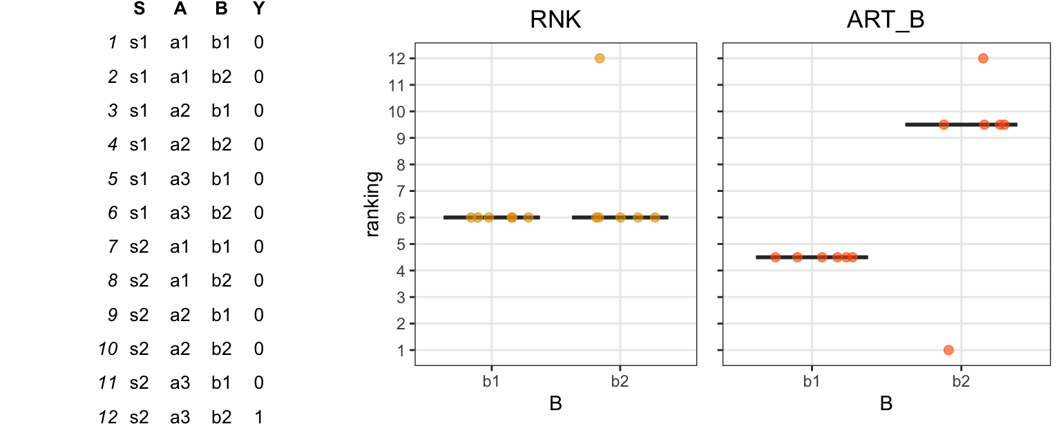
As discussed earlier, Lüpsen (2017) found that ART frequently fails when responses are discrete. The problem becomes more pronounced for variables with few discrete levels and as the sample size increases. The author provides a detailed analysis of why this happens, summarized as follows:

“There is an explanation for the increase of the type I error rate when the number of distinct values gets smaller or the sample size larger: due to the subtraction of the other effects — a linear combination of the means — from the observed values even tiny differences between the means lead to large differences in the ranking” (Lüpsen 2017).

Figure 8 illustrates this problem using a simple dataset with a binary variable. In our example, all but one value are zero. Notice how dramatically ART alters the ranks and exaggerates the difference between the two levels of \(B\) (\(b_1\) vs. \(b_2\)). This issue persists even when a large number of participants are added and there is only a single value of 1 among thousands of 0s, causing the method to produce arbitrarily low p-values. Then, a single value variation (e.g., turning this 1 to 0) will cause ART’s results to drastically change. Although this example illustrates an extreme case, ART’s instability can manifest in various forms, inflating error rates even when responses span a wider range of discrete values.

Figure 8: Results from an experiment following a \(3 \times 2\) design, where the response variable \(Y\) is binary and indicates the presence of an error. The plots show the rankings produced by the simple rank transformation (RNK) and by ART for the second factor. The solid lines represent group medians.

4 Defining the null hypothesis of interest

Before comparing different statistical methods, it is essential to assess whether they are actually comparable. If two methods are not designed to test the same null hypothesis, then direct comparisons between them can be misleading. In what follows, we clarify the interpretation of main and interaction effects and explain how we address potential issues in our analysis.

Interpreting main effects

The traditional ANOVA is used to test differences between two or more means. However, nonparametric tests often target other population parameters. For example, the Wilcoxon sign-rank test is commonly described as a test of medians for paired samples (McDonald 2014) and is used when population means are not of interest, e.g., when population distributions are skewed. The Mann-Whitney U and the Kruskal–Wallis tests are used, instead, to assess whether two or more independent samples come from the same population, or more technically, whether the mean ranks of the groups are the same. They can be only interpreted as tests of medians under the strict assumption that the population distributions of all groups have identical shapes and scales (George W. Divine and Juarez-Colunga 2018).

Defining the null hypothesis of interest of a rank transformation is more challenging. Conover and Iman (1981) show that the simple rank transformation procedure (RNK) is equivalent to the Mann-Whitney U and Kruskal–Wallis tests for independent samples. For paired samples, however, it results in a new test, which is different from the Wilcoxon sign-rank test and the Friedman test. Defining the null hypothesis of interest of ART is even more challenging because of the hybrid nature of the method. In particular, while ART is a rank-based transformation procedure, it aligns data with respect to means, where alignment is performed independently for each group.

Dealing with interpretation issues. To avoid such interpretation issues, we focus — unless otherwise stated — on effects that apply monotonic transformations to population distributions. This also ensures a monotonic relationship between different measures of central tendency, such as medians and means (with the exception of the Cauchy distribution, where the mean is undefined). In other words, if a treatment increases the population mean, it will also increase the population median. We present an example in Figure 9. The figure shows two population distributions corresponding to the two intermediate levels of difficulty of our illustrative example (see Figure 1). We observe that the increased difficulty of the task translates both the population mean and the median to the right. In this case, we expect a statistical test to reject the null hypothesis, no matter whether it tests the population mean, the median, or the overall distribution shape.

Figure 9: Time distributions for two task populations with difficulty levels 2 and 3 (see Figure 1).

Interpreting interaction effects

The ART procedure was proposed as an alternative to the rank transformation (Conover and Iman 1981) for testing interactions. As Higgins, Blair, and Tashtoush (1990) explained, the rank transformation is nonlinear and, as a result, it changes the structure of interactions. Therefore, “interaction may exist in the transformed data but not in the original data, or vice versa” (Higgins, Blair, and Tashtoush 1990). Figure 10 demonstrates the problem. In this example, the data have been sampled from perfectly normal distributions with equal variances. We observe that while no interaction effect appears in the original data (lines are parallel), the rank transformation deforms the trend. In particular, differences are more pronounced for the middle points of the three-level factor (“medium difficulty”). The figure also shows that the inverse normal transformation also deforms the interaction but to a lesser extent. Note that the problem emerges when the main effect is strong on all interacting factors.

Figure 10: Visualization of interaction effect for a 3 \(\times\) 2 experimental design before and after applying the rank transformation and the inverse normal transformation (INT) on an example dataset (within-subject design, \(n = 20\)). All data points represent means.

ART aims to correct this problem. However, nonlinear transformations come into place in various ways in experimental designs (Loftus 1978; Wagenmakers et al. 2012). They can deform distributions, making the interpretation of observed effects especially challenging. Before presenting our experimental method, we discuss these problems and explain how our approach takes them into consideration.

Removable interactions. Let us take a different dataset from a fictional experiment (within-subject design with \(n = 24\)) that evaluates the performance of two techniques (Tech A and Tech B) under two task difficulty levels (easy vs. hard). The experiment, for example, could test a mobile typing task, where the levels of difficulty correspond to texts of different lengths (short vs. long) under two typing techniques (with vs. without auto-completion). We assume that the researchers measure two dependent variables: task-completion time and perceived performance, which is measured through a five-level ordinal scale (from “very quick” to “very slow”). In this example, the main effects of task difficulty and technique are large. It is less clear, however, whether there is also an interaction between the two factors.

Figure 11 visualizes the means for each combination of the levels of the factors and highlights the possible interactions. Let us first concentrate on the first two plots that present results for the time measure. The trends in the left plot indicate an interaction effect, since the two lines seem to diverge as the task difficulty increases.

Figure 11: The line charts visualize the effects of task difficulty (easy vs. hard) and technique (Tech A vs. Tech B) for two measures: task completion time (left and middle) and perceived performance (right). All data points represent group means.

But how meaningful is this interpretation of interaction? As we dicussed earlier, time measurements are often taken from skewed distributions where the variance is not constant. Therefore, large effects are harder to observe in quick tasks than in slow ones. However, such trends do not necessarily reveal any real interactions, because they are simply due to observations at different time scales. Figure 11 (middle) visualizes the effects using a logarithmic scale. Notice that the lines in the plot are now almost parallel, suggesting no interaction effect.

The concept of removable or uninterpretable interactions, that is, interactions that disappear after applying a monotonic nonlinear transformation, was introduced by Loftus (1978). Over three decades later, Wagenmakers et al. (2012) revisited this work and found that psychology researchers are largely unaware of the concept, drawing incorrect conclusions about psychological effects on the basis of meaningless interactions.

This issue also extends to data collected from questionnaires. The right plot in Figure 11 shows results for perceived performance. Again, the line trends suggest an interaction effect. Unfortunately, the scale is ordinal, which means that distances between the five levels of the scale may not be perceived as equal by people. Furthermore, the scale is bounded, so the reason that the two lines are not parallel might be simply due to the absence of additional levels beyond the extreme “very slow” ranking. Concluding that there is a meaningful interaction here could be incorrect. Liddell and Kruschke (2018) extensively discuss how ordinal scales deform interactions.

Formal testing. We now formally test the above interactions by using ANOVA with different transformation methods. Below, we present the p-value returned by each method for task-completion time:

p-values for interaction effect on task-completion time

PAR	LOG	ART	RNK	INT
\(.023\)	\(.67\)	\(.00073\)	\(.66\)	\(.67\)

We observe that RNK and INT lead to p-values very close to the p-value of LOG, which suggests a similar interpretation of interaction effects. In contrast, ART returns a very low p-value (lower than the p-value of the regular ANOVA), indicating a different interpretation.

We also test the interaction effect on the ordinal dependent variable:

p-values for interaction effect on perceived performance

PAR	ART	RNK	INT	ATS
\(.0020\)	\(.00075\)	\(.0067\)	\(.0037\)	\(.0081\)

Notice that we omit the log-transformation method (LOG), as it is not relevant in this context. Instead, we conduct an analysis with the nonparametric ATS method (Brunner and Puri 2001), as implemented in the R package nparLD (Noguchi et al. 2012). All p-values are low, suggesting that an interaction effect exists. However, if we conduct a more appropriate analysis using an ordered probit model (Bürkner and Vuorre 2019; Christensen 2023), we find no supportive evidence for such an effect (check our analysis in the supplementary material).

In conclusion, focusing solely on the issues with the rank tranformation illustrated in Figure 10 is akin to missing the forest for the trees. When parallel main effects are present, interpreting interactions can be challenging for all methods — and ART offers no solution to this problem.

Disagreement on the interpretation of effects in GLMs

We further discuss interpetation issues in the broader context of generalized linear models (GLMs).

GLMs are defined by a link function \(g\) that connects a variable — linearly defined by the predictors — to a response variable \(Y\), which is assumed to be generated from a distribution in an exponential family. Exponential families include a wide range of common distributions, such as the normal, log-normal, exponential, binomial, and Poisson distributions.

For an experimental design with two factors, \(x_1\) and \(x_2\), the expected value (or mean) of \(Y\) conditional on \(x_1\) and \(x_2\) is expressed as follows: \[ E[Y|x_1, x_2] = g^{-1}(a_0 + a_1 x_1 + a_2 x_2 + a_{12}x_1 x_2) \tag{4}\] where \(g^{-1}\) is the inverse of the link function.

Statistical procedures based on GLMs define effects in terms of the coefficients \(a_{1}\), \(a_{2}\), and \(a_{12}\) in the linear component of the model. That is, the null hypothesis should be rejected when the corresponding coefficient (e.g., the coefficient \(a_{12}\) for the interaction) is non-zero. However, there is no consensus among researchers on this approach. We clarify the debate and explain how we address it.

Defining interactions on the scale of the response variable. Ai and Norton (2003) and, more recently, McCabe et al. (2022) show that the interaction coefficient alone is not sufficient to describe the actual interaction trend on the natural scale of the response variable. They argue that an interaction effect should instead be defined as the observed change in the marginal effect of \(x_1\) as a function of \(x_2\). Thus, the trends shown in Figure 11 do represent interactions, since the difference between Tech A and Tech B changes as a function of Difficulty on the original reponse scale (time or perceived performance).

Using this definition, the authors show that a zero interaction coefficient (\(a_{12} = 0\)) does not necessarily imply the absence of an interaction effect. In fact, for continuous predictors, they demonstrate that when \(a_{12} = 0\), the interaction effect can still emerge and is proportional to \(a_1\) and \(a_2\).

Responding to Ai and Norton (2003). Greene (2010) responds that the interpretation of Ai and Norton (2003) “produces generally uninformative and sometimes contradictory and misleading results” and instead advocates for using the model’s coefficients as the basis for inference:

“Statistical testing about the model specification is done at this step. Hypothesis tests are about model coefficients and about the structural aspects of the model specifications. Partial effects are neither coefficients nor elements of the specification of the model. They are implications of the specified and estimated model” (Greene 2010, 295).

Our position is fully aligned with Greene’s argument. As our earlier example (see Figure 11) demonstrates, interactions assessed on the scale of the response variable can be misleading about the true underlying effects that generated the data. How meaningful is it to declare interaction effects that arise solely from parallel main effects and lack any theoretical interpretation? It is worth noting that Ai and Norton (2003), as well as McCabe et al. (2022), overlook Loftus’ (1978) critique of uninterpretable interactions.

Nevertheless, in most of our experiments we select scenarios that avoid these interpretation problems, ensuring that the Type I error rates of the methods we compare do not depend on how one defines interactions. We clarify this point below.

Clarifying when the interpretation of effects becomes ambiguous. In nonlinear models, ambiguities in interpreting interaction effects arise when all relevant main effects are present — that is, when the coefficients of all interacting factors are non-zero. Interpretation issues may also extend to main effects when the interaction coefficient \(a_{12}\) is non-zero. In such cases, the marginal effect of a factor (e.g., \(x_1\)) may vary across levels of another factor even when its associated coefficient (e.g., \(a_1\)) is zero.

By contrast, interpretation is unambiguous in the following situations:

1. Main effects, when the interaction coefficient \(a_{12}\) is zero. In this case, if \(a_1 = 0\), then the factor \(x_1\) has no effect on the response scale. Likewise, if \(a_2 = 0\), then the factor \(x_2\) has no effect on the response scale.

2. Interaction effect, when either \(a_{1}\) or \(a_{2}\) is zero. In this case, if \(a_{12}=0\), then there is no interaction between \(x_1\) and \(x_2\) on the response scale.

Proofs of these statements are provided in Appendix II. In these scenarios, error rates are comparable across methods, regardless of whether the null hypothesis is defined in terms of the coefficients of the linear model or the observed effects on the response scale. For example, the divergence in ART’s results in our illustrative example (see Figure 1) cannot be attributed to interpretation issues, since the sample was drawn from a population with no effect of Technique (\(a_{1} = 0\)) and no interaction (\(a_{12}=0\)).

Throughout the remainder of the article, we explicitly distinguish between situations in which effect interpretation is unambiguous and those in which it is not. Because different methods may rely on different assumptions about the null hypothesis, we analyze ambiguous cases separately. However, we emphasize that the existing literature offers no guidance on how ART should be expected to behave when the definition of a main or interaction effect is ambiguous. Early evaluations of ART focused on linear models. Although Elkin et al. (2021) consider nonlinear models, they do not address how main and interaction effects should be interpreted when the definition of the null hypothesis depends on the scale of responses.

5 Experimental method

We can now detail our experimental method. We evaluate the standard parametric approach (PAR) and the three rank-transformation methods (RNK, INT, and ART) that we introduced earlier. We conduct a series of Monte Carlo experiments that assess their performance under a variety of experimental configurations.

Distributions. We evaluate both ratio and ordinal data, drawn from the following distributions:

1. Normal distribution \(\mathcal{N}(\mu, \sigma^2)\), where \(\mu\) is its mean and \(\sigma\) is its standard deviation. For most experiments where variances are equal, we set \(\sigma = 1\).
2. Log-normal distribution \(\mathcal{LogN}(\mu, \sigma^2)\), where \(\mu\) is its mean and \(\sigma\) is its standard deviation at the logarithmic scale. The log-normal distribution is a good model for various measures bounded by zero, such as task-completion times. We set \(\sigma = 1\) in our main experiments but evaluate a wider range of parameters in Appendix I.
3. Exponential distribution \(Exp(\lambda)\), where \(\lambda\) is its rate. The exponential distribution naturally emerges when describing the time elapsed between events. For example, we could use it to model the time a random person spends with a public display, or the waiting time before a new person approaches to interact with the display, when the average waiting time is \(\frac{1}{\lambda}\).
   
4. Cauchy distribution \(\mathcal{Cauchy}(x_0, \gamma)\), where \(x_0\) defines its location (median) and \(\gamma\) defines its scale. The Cauchy distribution is the distribution of the ratio of two independent normally distributed random variables. It rarely emerges in practice. However, it is commonly used in statistics to test the robustness of statistical procedures because both its mean and variance are undefined. As we discussed earlier, past evaluations of ART (Mansouri and Chang 1995; Elkin et al. 2021) show that the method fails under the Cauchy distribution. We set \(\gamma = 1\).
5. Poisson distribution \(\mathcal{Pois}(\lambda)\), where \(\lambda\) is its rate. It expresses the probability of a given number of events in a fixed interval of time. For example, we could use it to model the number of people who interact with a public display in an hour, when the average rate is \(\lambda\) people per hour.
6. Binomial distribution \(\mathcal{B}(\kappa, p)\), where \(\kappa\) defines the number of independent Bernoulli trials and \(p\) is the probability of error or success of each trial. It frequently appears in HCI research, as it can model the number of successes and failures in a series of experimental tasks. We set \(\kappa = 10\) in our main experiments but evaluate a wider range of parameters in Appendix I.
7. Distributions of Likert-item responses with 5, 7, and 11 discrete levels.

Experimental designs. We present results for five experimental designs. To simplify our presentation, we start with (i) a 4 \(\times\) 3 within-subject factorial design. We then show how our conclusions generalize to four additional designs: (ii) a 2 \(\times\) 3 between-subject design; (iii) a 2 \(\times\) 4 mixed design, with a between-subject factor and a within-subject factor; (iv) a 2 \(\times\) 2 \(\times\) 2 within-subject design; and (v) a 3 \(\times\) 3 \(\times\) 3 within-subject design.

Sample sizes. We focus on three sample sizes, \(n=10\), \(n=20\), and \(n=30\), where \(n\) represents the cell size in an experimental design. However, for certain scenarios, we also report results for larger sample sizes, up to \(n = 512\). In within-subject designs, where all factors are treated as repeated measures, \(n\) corresponds to the number of subjects \(N\) (commonly human participants in HCI research). In contrast, in a 2 \(\times\) 3 between-subject design, a cell size of \(n = 20\), implies a total of \(N = 120\) subjects.

Equal vs. unequal variances. For normal and ordinal distributions, we test the robustness of the methods when variances are unequal.

Evaluation measures. In addition to Type I error rates, we compare the statistical power of the methods and compare their effect size estimates with ground-truth estimates.

Magnitude of effects. We analyze both main and interaction effects, examining how increasing the magnitude of effect of one factor influences the Type I error rates of other factors and their interactions. In addition, we examine how increasing two main effects in parallel influences the Type I error rate of their interaction, while emphasizing that the definition of the null hypothesis in this case is ambiguous.

Previous evaluations of rank transformation methods (Beasley, Erickson, and Allison 2009; Lüpsen 2018) have also examined unbalanced designs, where cell sizes vary across the levels of a factor. When combined with unequal variances, such designs often pose challenges for both parametric procedures (Blanca et al. 2018) and rank transformation methods (Beasley, Erickson, and Allison 2009; Lüpsen 2018). As noted earlier, we do not consider unbalanced designs in our main article. However, we provide additional experimental results on missing data in Appendix I.

Statistical modeling

For simplicity, we explain here our modeling approach for two factors, but its extension to three factors is straightforward.

Linear component. The base of our data generation process for all distributions is the following linear predictor:

\[ \ell_{ijk} = \mu + s_k + a_1 x_{1i} + a_2 x_{2j} + a_{12} x_{1i} x_{2j} \tag{5}\]

• \(\mu\) is the intercept

• \(s_k \sim \mathcal{N}(0, \sigma_s^2)\) is the random intercept effect of the k-th subject, where \(k = 1..n\)

• \(x_{1i}\) is a numerical encoding of the i-th level of factor \(X_1\), where \(i = 1..m_1\)

• \(x_{2j}\) is a numerical encoding of the j-th level of factor \(X_2\), where \(j = 1..m_2\)

• \(a_1\), \(a_2\), and \(a_{12}\) express the magnitude of main and interaction effects

While random slope effects can have an impact on real experimental data (Barr et al. 2013), we do not consider them here for two main reasons: (1) to be consistent with previous evaluations of the ART procedure (Elkin et al. 2021); and (2) because mixed-effects procedures with random slope effects are computationally demanding, adding strain to simulation resources. However, there is no good reason to believe that adding random slope effects would impact our findings and conclusions.

Encoding the levels of factors. To encode the levels of the two factors \(x_{1i} \in X_1\) and \(x_{2j} \in X_2\) we proceed as follows:

1. We normalize the distance between their first and their second levels, such that \(x_{12} - x_{11} = 1\) and \(x_{22} - x_{21} = 1\). This approach enables us to conveniently control for the main and interaction effects by simply varying the parameters \(a_1\), \(a_2\), and \(a_{12}\).

2. For the remaining levels, we randomly sample from a uniform distribution that spans the range between these two extreme levels, i.e., between \(x_{11}\) and \(x_{12}\) for \(X_1\), and between \(x_{21}\) and \(x_{22}\) for \(X_2\). This approach allows us to generate and evaluate a substantial variety of configurations, each representing different relative effects between levels.

3. We require all levels to sum up to 0, or \(\sum\limits_{i=1}^{m_1} x_{1i} = 0\) and \(\sum\limits_{j=1}^{m_2} x_{2j} = 0\), which ensures that the grand mean is \(\mu\).

For example, we can encode a factor with four levels as \(\{-.6, .4, .1, .1\}\) or as \(\{-.5, .5, .3, -.3\}\).

Generating ratio data. We generate ratio-scaled data using generalized linear modeling (Bolker et al. 2009). Specifically, we use an inverse link function \(g^{-1}\) to relate the linear predictor \(\ell_{ijk}\) to the location parameter of the target distribution:
\[ Y_{ijk} \sim \mathcal{F}(location=g^{-1}(\ell_{ijk}), ...) \tag{6}\]

where \(\mathcal{F}\) denotes the probability density (or mass) function from which the responses \(Y_{ijk}\) are drawn. For example, the mean of the exponential distribution is equal to \(1 / \lambda\), where \(\lambda\) is its rate parameter. This mean is linked to the linear predictor through the inverse link function \(g^{-1}(x) = e^{x}\), which implies \(\lambda = e^{-\ell_{ijk}}\). Similarly, for the binomial distribution, the canonical link function is the logit function, whose inverse is the logistic function \(g^{-1}(x) = 1 / (1 + e^{-x})\).

Table 1 summarizes how the location parameters of all the distributions are linked to the linear predictor. We emphasize that the Cauchy distribution does not define a generalized linear model (because it does not belong to an exponential family) but we nevertheless use a model that links its location (the median) to the linear predictor via the identity link.

Table 1: Distribution parameters and their links to the linear predictor \(\ell_{ijk}\)

distribution	location parameter	description
Normal	\(\mu = \ell_{ijk}\)	mean
Log-normal	\(\mu = \ell_{ijk}\)	mean at logarithmic scale (logarithm of median)
Exponential	\(\lambda = e^{-\ell_{ijk}}\)	rate (1 / mean)
Cauchy	\(x_0 = \ell_{ijk}\)	median
Poisson	\(\lambda = e^{\ell_{ijk}}\)	rate (mean)
Binomial	\(p = 1 / (1 + e^{-\ell_{ijk}})\)	probability of success or error

Generating ordinal data. For generating ordinal data, we follow a latent-variable approach as explained by Liddell and Kruschke (2018). Specifically, we consider that there is a continuous latent variable that follows a normal distribution: \[ Y_{ijk}^* \sim \mathcal{N}(\mu = \ell_{ijk}, \sigma^2 = 1) \tag{7}\] From this, we derive discrete responses \(d = 1,2 ... D\) by applying fixed thresholds \(\tau_d \in (-\infty, \infty)\) as follows: \[ \begin{aligned} Y_{ijk} = d\ \ \text{if}\ \ \tau_{d-1} < Y_{ijk}^* \leq \tau_d \end{aligned} \tag{8}\] Since, in practice, \(\tau_0 = -\infty\) and \(\tau_D = \infty\), generating responses with \(D\) discrete levels requires \(D-1\) thresholds.

Effects and population control

We next detail how we select the parameters of the linear component (see Equation 5) for the various distributions, as well as the thresholds of the ordinal model (see Equation 8).

Magnitude of effects. We control the magnitude of effects by varying \(a_1\), \(a_2\), and, for some experiments (those evaluating power for interactions), \(a_{12}\). Figure 12 presents normal distributions (\(\sigma = 1\)) generated across the range of values of \(a_1\) used to evaluate Type I error rates. In these examples, we illustrate effects for a factor with three categorical levels and, for clarity, disregard between-subject variability (\(\sigma_s = 0\)).

Figure 12: Varying \(a_1\) to control the magnitude of the main effect of \(X_1\). The plots show examples of normal distributions (\(\sigma = 1\)) for a factor with three categorical levels.

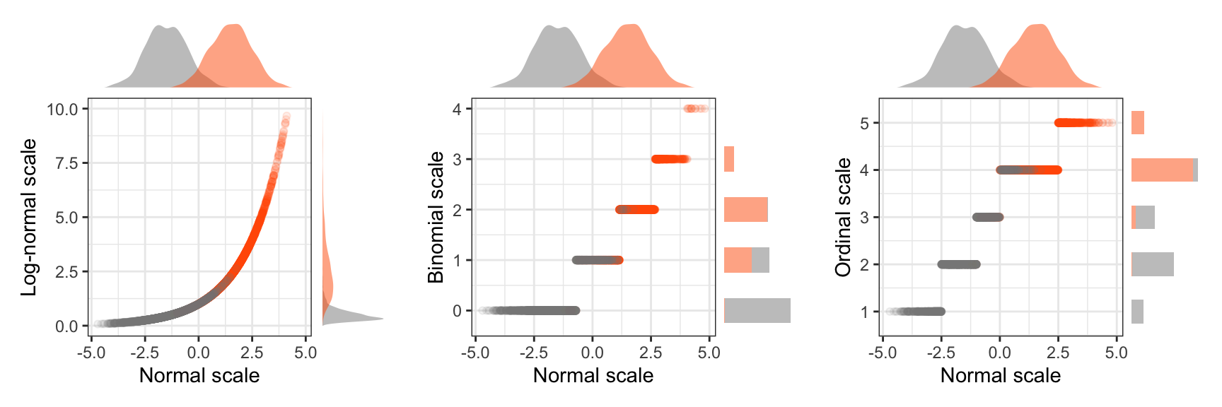
Intercept and variance parameters. Fixing the intercept \(\mu\) directly in a nonlinear model generally leads to arbitrary population-level response distributions, because the marginal mean depends on the link function, the response distribution, the variance of the random effects, and the magnitude of the fixed effects. We therefore calibrate the intercept \(\mu\) so that the induced location of the responses matches a pre-specified target value. Table 2 reports the target location for each distribution, which is typically the overall mean in all cases except for the Cauchy distribution, where the median is used. We detail how \(\mu\) is analytically derived from these target values in Appendix II.

Table 2: Target mean (median for the Cauchy distribution) of responses \(Y_{ijk}\)

Normal	Log-normal	Exponential	Cauchy	Poisson	Binomial	Ordinal
0	1	0.5	0	3	0.1 (per trial)	0

Figure 13 shows distributions generated with these location values when \(a_1 = 2\) for a factor with three categorical levels.

Figure 13: Different ratio distributions generated with \(a_1 = 2\) when \(X_1\) has three categorical levels (here, \(\sigma_s = 0\)).

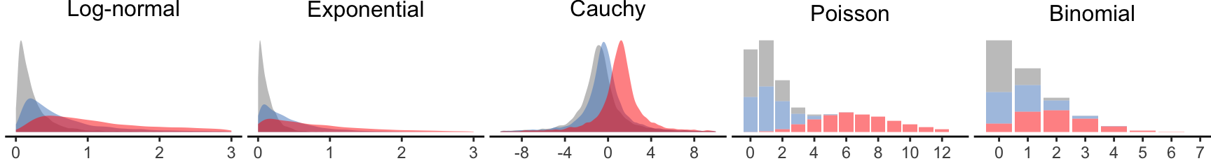
In practice, we randomly choose the standard deviation \(\sigma_s\) — which determines between-subject variability — from the interval \([0.1, 0.5]\), drawing each value from a uniform distribution.

Thresholds for ordinal scales. For ordinal data, we evaluate \(D =\) 5, 7, or 11 discrete levels. To derive the discretization thresholds \(\tau_d\), we first consider the range \([-2SD, 2SD]\) , where \(SD\) is the overall standard deviation of the latent variable \(Y^{*}_{ijk}\). We then divide this range into 5, 7, or 11 intervals, following two different strategies: (i) setting thresholds to be equidistant; or (ii) considering flexible thresholds, randomly drawing their position in the above range.

Figure 14 presents examples of equidistant and flexible thresholds for a 5-level scale when the magnitude of main effect of \(X_1\) is either \(a_1 = 2\) or \(a_1 = 8\), while all other effects are zero.

Figure 14: The four vertical lines in each plot represent thresholds defining 5-level ordinal scales. Thresholds are either equidistant (top) or flexible (bottom) within a range of \(\pm 2\) standard deviations around the grand mean \(\mu = 0\).

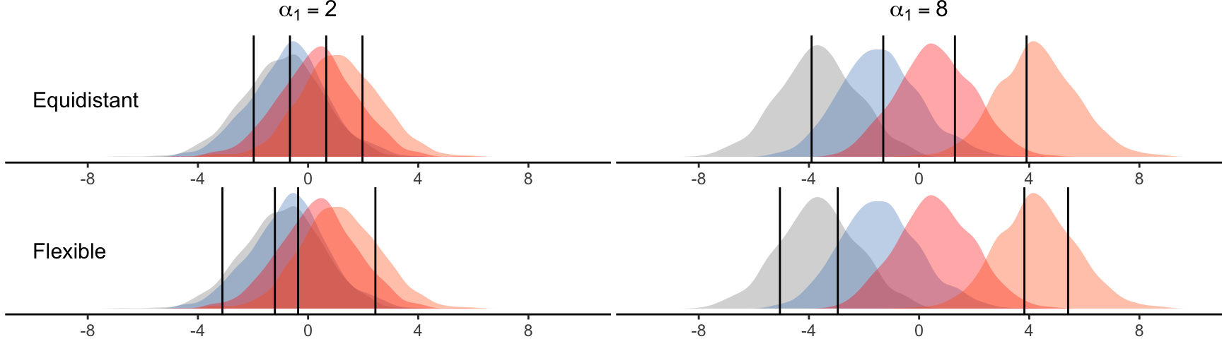
Implementation of rank transformation methods

For the aligned rank transformation (ART), we use the R implementation of ARTool v0.11.1 (Kay et al. 2021). For the pure rank transformation (RNK), we use R’s rank() function. We use the Rankit formulation (Bliss, Greenwood, and White 1956) for the inverse normal transformation (INT), as explained earlier.

Unless stated otherwise, we analyze the data using ANOVA with R’s aov() function and the model specification Y' ~ X1 * X2 + Error(S). For balanced designs, this approach yields results that are identical or nearly identical to those obtained using R’s lmer() function with the model specification Y' ~ X1 * X2 + (1 | S).

Evaluation measures

Significance tests have two types of errors. Type I errors, or false positives, are mistaken rejections of the null hypothesis. Type II errors, of false negatives, are failures to reject a null hypothesis that is actually true. In our illustrative example in Figure 1, a Type I error is finding that there is an effect of the choice of the technique on time performance. A Type II error, in turn, is finding that the task difficulty has no effect on time performance.

Statistical significance testing requires setting a significance threshold known as significance or \(\alpha\) (alpha) level, with typical values \(\alpha = .05\) and \(\alpha = .01\). The Type I error rate of a well-behaved significance test should be close to this nominal alpha level. An error rate clearly above this level suggests that the significance test is too liberal, while an error rate clearly below this level suggests that the test is too conservative. We test two significance levels: \(\alpha = .05\) and \(\alpha = .01\). For brevity, we report only the results for \(\alpha = .05\) and include additional results in Appendix I and our supplementary material.

When the null hypothesis is ambiguous, we report positive rates, noting that their interpretation as Type I error rates depends on how the null hypothesis is defined. Nevertheless, we generally recommend Greene’s (2010) interpretation, which is based on the coefficients of the underlying model.

We do not directly evaluate Type II errors. Instead, we report on statistical power defined as \(Power = 1 - \beta\), where \(\beta\) is the rate of Type II errors. Significance tests do not provide any power guarantees. However, we can compare the power of different methods to evaluate their relative performance. For log-normal and ordinal distributions, we also assess effect size estimates, where we use as ground truth the estimates of a parametric ANOVA conducted either on the logarithmic scale of the data (for log-normal) or latent variable \(Y^*\) (for ordinal). While partial \(\eta^2\) is the most commonly used effect size measure, we also evaluate Cohen’s \(f\), as its expected value is proportional to the real magnitude of the effect. However, \(\eta^2\) can be directly derived from Cohen’s \(f\) as follows:

\[ \eta^2 = \frac{f^2}{1 + f^2} \tag{9}\]

Hardware platform and iterations

Our experimental R code is available in our supplementary material. We ran our experiments separately in a cluster of 8 machines Dell R640 Intel Xeon Silver 4112 2.6GHz with 4 cores and 64 GB memory. Our R code was parallelized to use all four cores of each machine.

To estimate the power and Type I error rates of the four methods with enough precision, we ran \(5000\) iterations for each population configuration and each sample size.

6 Results

Each experiment concentrated on a unique combination of distributions, experimental designs, and evaluation measures. We organize our results into several subsections, addressing both main and interaction effects.

Type I error rates in ratio scales

We first evaluate Type I error rates for ratio scales. We test a 4 \(\times\) 3 within-subject design, where we refer to the 4-level factor as \(X_1\) and the 3-level factor as \(X_2\). We encourage readers to use the interactive tools provided in the figures to explore the trends in greater detail.

Main effects. Figure 15 presents Type I error rates for the main effect of \(X_2\) as the magnitude of the main effect of \(X_1\) increases.

Figure 15: Type I error rates (\(\alpha = .05\)) for the main effect of \(X_2\) as a function of the magnitude \(a_1\) of the main effect of \(X_1\)

Overall, RNK and INT exhibit very good behavior across all distributions. The standard parametric ANOVA (PAR) maintains error rates below \(5\%\), but for some distributions (log-normal, Cauchy, and Poisson) the error rates are noticeably lower, suggesting a loss of statistical power. Consistent with previous findings (Mansouri and Chang 1995; Elkin et al. 2021), ART fails to control the Type I error rate under the Cauchy distribution. However, we further show that ART is also problematic for other non-normal distributions. As the main effect of the first factor \(X_1\) increases, Type I errors on the second factor \(X_2\) increase dramatically, approaching \(100\%\) when \(a_1=8\). For the binomial distribution, error rates are already elevated (\(\approx 9\%\) for \(n = 20\)) even when \(a_1=0\), and increase further as the sample size grows.

Contrasts. The same issues arise when running ART’s contrast procedure (Elkin et al. 2021). Figure 16 shows the corresponding results, where we report average error rates for three pairwise comparisons (since \(X_2\) has three levels). In the rest of the paper, we focus on overall effects, since the results for contrasts exhibit the same patterns.

Figure 16: Average Type I error rates (\(\alpha = .05\)) for contrasts on factor \(X_2\) as a function of the magnitude \(a_1\) of the main effect of \(X_1\)

Interaction effects. Figure 17 presents Type I error rates for the \(X_1 \times X_2\) interaction when \(a_2=0\) and \(a_1\) increases. Overall, we observe trends similar to those for main effects. ART again fails in comparable ways, although its error rates are slightly lower in this case. In addition, PAR tends to inflate error rates under the log-normal and exponential distributions as \(a_1\) increases.

Figure 17: Type I error rates (\(\alpha = .05\)) for the interaction \(X_1 \times X_2\) as a function of the magnitude \(a_1\) of the main effect of \(X_1\)

The scenarios above do not capture the failure cases of the rank transformation discussed earlier (see Figure 10), as these arise only when both coefficients \(a_1\) and \(a_2\) are non-zero. Because multiple definitions of interaction effects are possible in such cases, we address them in a separate subsection.

Analysis for large samples. We also examine Type I error rates for larger sample sizes (up to \(n=512\)), fixing \(a_1=1\). As shown in Figure 18, ART’s error rates increase only slightly for log-normal data but rise substantially under the Cauchy, Poisson, and binomial distributions. These patters are consistent for both the main effect of \(X_2\) and the interaction effect. As we later observe for ordinal scales, ART’s tendency for increasing Type I error rates with sample size appears to be a more general issue for discrete distributions.

Figure 18: Type I error rates (\(\alpha = .05\)) for the main effect of \(X_2\) and the interaction \(X_1 \times X_2\) as a function of the size \(n\) of the sample. The effect on \(X_1\) is non-null, where we set \(a_1 = 1\).

Type I error rates in ordinal scales

We also evaluate Type I error rates for ordinal scales. We test again a \(4 \times 3\) repeated-measures design.

Main effects. Figure 19 present Type I errors for \(X_2\)’s main effect, as we vary \(X_1\)’s magnitude of main effect.

Figure 19: Type I error rates (\(\alpha = .05\)) for the main effect of \(X_2\) as a function of the magnitude \(a_1\) of the main effect of \(X_1\)

Our results indicate that PAR, RNK, and INT consistently maintain error rates close to \(5\%\) across all tested ordinal scales. In contrast, ART exhibits a significant inflation of error rates, although this issue becomes less severe when the number of levels increases. Notably, error rates are more pronounced for flexible thresholds and tend to increase with sample size.

Interaction effects. Figure 20 displays error rates for the interaction \(X_1 \times X_2\) with a single main effect applied to \(X_1\). The observed patterns align with our previous findings; ART consistently inflates error rates.

Figure 20: Type I error rates (\(\alpha = .05\)) for the interaction \(X_1 \times X_2\) as a function of the magnitude \(a_1\) of the main effect of \(X_1\)

Analysis for large samples. Let us further explore ART’s error rates when sample sizes become larger. As shown in Figure 21, error rates explode even when all population effects are null. The patterns are similar for all three effects.

Figure 21: Type I error rates (\(\alpha = .05\)) as a function of the size \(n\) of the sample, where all population effects are null.

Type I errors across experimental designs

We examine the generalizability of the preceding results across alternative experimental designs involving two or three factors. We assess five of the six ratio-scale distributions considered earlier, excluding the Cauchy distribution and replacing it with a 5-level ordinal scale with flexible thresholds.

Main effects. Figure 22 illustrates Type I error rates for the main effect of \(X_2\) while varying the magnitude of the main effect of \(X_1\), focusing on \(n = 20\). RNK and INT consistently maintain error rates close to \(5\%\), with the exception of the Poisson distribution, for which error rates become low in the two within-subject designs (particularly for INT). Similarly, PAR generally maintains error rates near \(5\%\), but they drop to notably low levels for certain combinations of designs (\(2 \times 2 \times 2\) and \(3 \times 3 \times 3\) within subjects) and distributions (log-normal and exponential).

In contrast, ART inflates error rates across all non-normal distributions, with the extent of inflation varying by design. For example, ART performs particularly poorly for the ordinal scale when applied to the \(2 \times 2 \times 2\) and \(3 \times 3 \times 3\) designs. In these designs, we also observe inflated error rates for log-normal data, even when \(a_1 = 0\).

Figure 22: Type I error rates (\(\alpha = .05\)) for the main effect of \(X_2\) as a function of the magnitude \(a_1\) of the main effect of \(X_1\) (\(n = 20\))

Interaction effects. Figure 23 displays Type I error rates for the interaction effect \(X_1 \times X_2\) while varying the effect of \(X_1\) (\(n = 20\)). We observe consistent trends in line with our previous findings. For additional insights, we direct readers to our raw experimental data, which demonstrate that these trends persist across other interaction terms, namely \(X_1 \times X_3\), \(X_2 \times X_3\), and \(X_1 \times X_2 \times X_3\), within the two 3-factor designs.

Figure 23: Type I error rates (\(\alpha = .05\)) for the interaction \(X_1 \times X_2\) as a function of the magnitude \(a_1\) of the main effect of \(X_1\) (\(n = 20\))

Interactions under parallel main effects

Let us now examine interaction effects when both coefficients \(a_1\) and \(a_2\) increase in parallel. In this scenario, the interpretation of an interaction effect becomes ambiguous in nonlinear models. Therefore, we refrain from labeling positive rates as Type I error rates. However, if the null hypothesis is defined in terms of the coefficients of the linear component of the model (see Equation 5), following the recommendation of Greene (2010) — that is, \(a_{12} = 0\) — then all these values can be interpreted as Type I error rates.

Ratio scales. Figure 24 presents results for ratio scales.

Figure 24: Positive rates (\(\alpha = .05\)) for the interaction \(X_1 \times X_2\) as a function of the magnitudes \(a_1 = a_2\) of the main effects of \(X_1\) and \(X_2\). Note: These values correspond to Type I error rates under the null hypothesis \(a_{12} = 0\); alternative definitions of the null hypothesis may lead to different results.

Positive rates become exceptionally high in many cases, reaching up to 100%. These results require careful interpretation. As discussed in Section 4, interaction effects in nonlinear models can be interpreted in two distinct ways, and the results produced by the different methods are not always consistent with our chosen definition. We therefore examine the outcomes for each method in turn:

• PAR. Positive rates are high for all non-normal distributions (with the exception of the Cauchy distribution) and increase further as sample size grows. This behavior arises because the null hypothesis for this method is defined on the scale of the response variable, rather than on the scale of the linear model.

• RNK. Positive rates increase dramatically once main effects exceed a certain magnitude. This well-known issue stems from the way rank transformations distort interaction effects (see Figure 10), even when the underlying distributions are normal.

• INT. It performs better than RNK in continuous distributions, with rates increasing only when \(a_1\) and \(a_2\) become large. However, under the Poisson and binomial distributions, INT performs worse than RNK. Interestingly, INT is particularly robust under the Cauchy distribution.

• ART. ART maintains correct positive rates only when the population distributions are normal. For all other distributions, rates increase rapidly as effect sizes grow. Two factors may account for this behavior: (i) a lack of robustness to violations of the method’s assumptions, as also observed in our earlier experiments; and (ii) issues related to interaction interpretation. These findings confirm that ART is not scale-invariant and interprets interactions relative to the scale of the observed data.

Ordinal scales. Figure 25 presents our results for ordinal data. No method maintains low positive rates under all conditions. We note that ART consistently performs worse than PAR. INT performs worse than ART and PAR in one specific case (\(a_2, a_2 = 8\) in a scale with 11 equidistant levels), but overall, it exhibits a better behavior than all other methods. Once again, the high positive rates can be partly explained by insufficient statistical robustness and ambiguities in how the methods interpret interaction effects.

Figure 25: Positive rates (\(\alpha = .05\)) for the interaction \(X_1 \times X_2\) as a function of the magnitudes \(a_1 = a_2\) of the main effects of \(X_1\) and \(X_2\). Note: These values correspond to Type I error rates under the null hypothesis \(a_{12} = 0\); alternative definitions of the null hypothesis may lead to different results.

Other designs. Our findings in Figure 26 further demonstrate that all methods struggle to accurately detect interactions. INT shows unusually low rates in certain configurations (e.g., \(2 \times 3\) and \(2 \times 2 \times 2\)), suggesting potential difficulty in detecting subtle interaction effects when main effects are large. RNK displays a similar pattern for the \(2 \times 2 \times 2\) design. In addition, both RNK and INT exhibit higher rates under discrete distributions, in some cases exceeding those observed for ART.

Figure 26: Positive rates (\(\alpha = .05\)) for the interaction \(X_1 \times X_2\) as a function of the magnitudes \(a_1 = a_2\) of the main effects of \(X_1\) and \(X_2\) (\(n = 20\)). Note: These values correspond to Type I error rates under the null hypothesis \(a_{12} = 0\); alternative definitions of the null hypothesis may lead to different results.

These results illustrate the complexity and pitfalls of interpreting interaction effects under assumption violations — regardless of the method used.

Type I errors under unequal variances

Many statistical procedures assume equal variances across all levels of each independent variable, or more strictly, across all possible pairs of factor levels (the latter is known as the sphericity assumption in repeated-measures ANOVA). Nonparametric tests are often mistakenly assumed to be free of such assumptions; however, as discussed earlier, this is generally incorrect.

Our next experiment evaluates the behavior of the four methods under conditions of unequal variances, focusing on the normal distribution and four ordinal distributions. For ordinal outcomes, we control variances at the level of the latent variable \(Y^*\).

We examine three two-factor designs: (i) a \(4 \times 3\) within-subject design; (ii) a \(2 \times 3\) between-subject design; and (iii) a \(2 \times 4\) mixed design. We set all effects to zero and vary the ratio \(r _{sd}\) of standard deviations between the levels of the first factor \(X_1\). Figure 27 shows the five ratios tested when \(X_1\) has two levels. When \(X_1\) has additional levels (as in the \(4 \times 3\) design), their standard deviations are randomly drawn from a range bounded by the standard deviations of the first two levels.

Figure 27: Varying the ratio \(r _{sd}\) of standard deviations across the levels of \(X_1\). The plots show examples of population distributions for factors with two categorical levels.

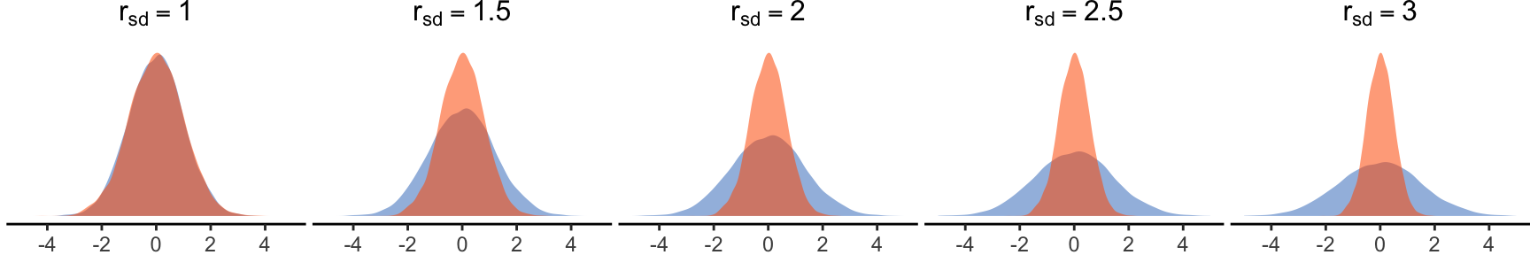
Main effects. We begin by investigating how the four methods detect main effects of \(X_1\). Interpreting results in this setting is challenging because the underlying populations differ in variance while sharing the same means (and medians). For ordinal scales, differences in variance may also manifest as differences in observed means (Liddell and Kruschke 2018). To highlight these interpretation issues, we therefore label the observed rates of positives as Positives (%). These rates can nonetheless be interpreted as Type I error rates if the null hypothesis is defined in terms of mean differences on the latent variable.

Figure 28 presents the results. Under normal distributions, and depending on the experimental design, the different methods either slightly inflate or slightly deflate the positive rates as \(r _{sd}\) increases, with no method clearly outperforming the others. For ordinal scales, larger values of \(r _{sd}\) primarily affect conditions with flexible thresholds. This effect is particularly pronounced for PAR, although all methods are affected.

Figure 28: Positive rates (\(\alpha = .05\)) for the main effect of \(X_1\) as the ratio of standard deviations \(r _{sd}\) for \(X_1\) increases (\(n=20\)). Note: When \(r _{sd} > 1\), the underlying populations are no longer identical, and different interpretations of the null hypothesis may lead to different outcomes.

We also examine the influence of unequal variances across the levels of \(X_1\) on the Type I error rate for \(X_2\), as shown in Figure 29. In this case, there is no ambiguity in the interpretation of effects because the populations defined by \(X_2\) are identical.

The Type I error rates of PAR, RNK, and INT appear largely unaffected by increases in \(r _{sd}\). In contrast, ART yields high error rates, surpassing acceptable levels even under normal distributions (see, for example, the \(2 \times 4\) mixed design). Thus, unequal variances pose a more serious problem for ART than for the other methods, as the method’s sensitivity propagates across factors. This provides further evidence that ART’s alignment procedure leads to confounding across effects.

Figure 29: Type I error rates (\(\alpha = .05\)) for the main effect of \(X_2\) as the ratio of standard deviations \(r _{sd}\) across the levels of \(X_1\) increases (\(n=20\))

Interaction effects. Finally, we evaluate Type I error rates for the interaction, as shown in Figure 30. ART exhibits a similar pattern as before, with error rates increasing as \(r _{sd}\) grows. We also observe some inflation of Type I error rates for the other three methods under the \(4 \times 3\) within-subject design, albeit to a significantly lesser degree.

Figure 30: Type I error rates (\(\alpha = .05\)) for the interaction effect \(X_1 \times X_2\) as the ratio of standard deviations \(r _{sd}\) across the levels of \(X_1\) increases (\(n=20\))

Statistical power

We evaluate the statistical power of the four methods on the three two-factor designs. Because there is a tradeoff between Type I and Type II errors, high power may simply reflect an inflated Type I error rate. Since a main effect on \(X_1\) inflates ART’s Type I error rates for \(X_2\) and for their interaction (see previous sections), we therefore focus on single-effect scenarios.

Main effects. We vary the magnitude of effect on \(X_1\) and \(X_2\) separately and assess each method’s power to detect the corresponding effect at \(\alpha = .05\). Specifically, we manipulate the parameters \(a_1\) or \(a_2\) over the range \(0.2\) to \(0.8\). Depending on the experimental design, this range allows us to simulate both low-power settings (e.g., power below \(30\%\)) and high-power settings (e.g., power above \(80\%\)).

Figure 31 presents the results for \(X_1\). In many configurations, differences in power across methods are modest. To facilitate comparison, we also report method rankings; readers are encouraged to interact with the figures for precise power estimates.

PAR achieves the highest power under the normal and exponential distributions, but its power is particularly low under the log-normal distribution. ART initially appears advantageous under the log-normal, binomial, and ordinal distributions for small effects, likely reflecting inflated Type I errors under these conditions. As \(a_1\) grows larger, ART’s relative advantage diminishes, and it ultimately becomes the least powerful method. Finally, INT consistently outperforms RNK and ranks highly across all conditions.

Figure 31: Power (\(\alpha = .05\)) for detecting the main effect of \(X_1\) as a function of its magnitude \(a_1\), with \(n=20\).

Figure 32 presents our results for \(X_2\). Because this factor has a different number of levels across designs, we assess different ranges of power for each design. Nevertheless, the same overall patterns emerge.

Figure 32: Power (\(\alpha = .05\)) for detecting the main effect of \(X_2\) as a function of its magnitude \(a_2\), with \(n=20\).

Interaction effects. We also vary the magnitude of the interaction effect \(X_1 \times X_2\) by manipulating the parameter \(a_{12}\) over the range \(0.5\) to \(2.0\), and then measure the power to detect this interaction. The results, summarized in Figure 33, are consistent with the patterns observed for main effects.

Figure 33: Power (\(\alpha = .05\)) for detecting the interaction effect \(X_1 \times X_2\) as a function of its magnitude \(a_{12}\), with \(n=20\).

Overall, there is no clear winner, but we observe that PAR shows poor power performance for log-normal data, while INT consistently outperforms RNK. Furthermore, ART provides no substantial power advantage, despite its inflated Type I error rates.

Effect size estimates

Transformations — even monotonic ones — alter both the absolute magnitude of effects and the total variance of the data. A natural question, therefore, is how to interpret effect size estimates derived from rank transformations and whether such estimates are meaningful and comparable across methods. Nevertheless, Kay (2025) provides a tutorial for deriving standardized effect sizes from ART, and many of the papers we reviewed report such estimates. This practice motivates a more systematic investigation.

Log-normal distributions. We begin by examining log-normal responses. Consider a \(4 \times 3\) within-subject design with \(n = 20\), in which the effect of the first factor \(X_1\) is null (\(a_1 = 0\)) and there is no interaction (\(a_{12} = 0\)). Figure 34 displays the partial \(\eta^2\) estimates produced by each method for the effect of \(X_1\) as the magnitude of the effect on the second factor \(X_2\) increases. These estimates are compared to those from a ground-truth analysis, defined here as ANOVA applied to the log-transformed responses.

Figure 34: Boxplots summarizing the partial \(\eta^2\) estimates obtained with each method from 300 simulated datasets (\(n=20\)). The population effect of \(X1\) is null, and responses follow log-normal distributions. Hover over the plots to compare the methods.

We observe that ART is the only method for which the estimated effect sizes for \(X_1\) are influenced by the magnitude of the effect on \(X_2\). These results clearly demonstrate that ART’s alignment mechanism fails in nonlinear models with skewed distributions and leads to confounding across effects.

Figure 35 presents partial \(\eta^2\) estimates when the effect of \(X_1\) is no longer null (\(a_1 = 1\)). PAR performs poorly for these data, consistently underestimating effect sizes. ART also tends to underestimate effects when \(a_2 = 0\); however, as \(a_2\) increases, its estimates become more variable and exhibit an overall tendency to increase. RNK and INT yield the most precise estimates. INT is only mildly affected when \(a_2 = 8\).

Figure 35: Boxplots summarizing partial \(\eta^2\) estimates obtained with each method from 300 simulated datasets (\(n=20\)). The population effect of \(X1\) is non-null (\(a_1 = 1\)), and responses again follow log-normal distributions. Hover over the plots to compare the methods.

Systematic comparison to ground truth estimates. We conduct an additional experiment to compare the methods to the ground truth across a wider range of effect magnitudes for the normal, log-normal, and ordinal distributions (the latter with five levels and flexible thresholds). For ordinal data, the ground truth is defined as ANOVA applied to the latent variable (i.e., the data prior to discretization). We now use Cohen’s \(f\) as a measure of effect size, which is expected to be proportional to the true effect magnitude. Without loss of generality, we focus on the main effect of \(X_1\) and fix the sample size to \(n=20\).

Figure 36 illustrates the relationship between the Cohen’s \(f\) estimated by each method and the corresponding ground-truth estimate, as \(a_1\) and \(a_2\) vary independently within the range \([-2, 2]\). This produces Cohen’s \(f\) values between \(0\) and \(1\) for the \(4 \times 3\) within-subject and \(2 \times 3\) between-subject designs, and a wider range for the \(2 \times 4\) mixed design. Proximity to the black diagonal indicates closer agreement with the ground truth. Points above the diagonal indicate overestimation of the effect size, whereas points below indicate underestimation.

Figure 36: Scatterplots showing the relationship between effect size estimates (Cohen’s \(f\)) obtained with each method and those from the ground-truth analysis for the main effect of \(X_1\), when \(a_1\) and \(a_2\) vary independently within the range \([-2, 2]\).

Under log-normal distributions, PAR tends to severely underestimate effect sizes, whereas ART produces estimates that are widely dispersed on both sides of the ground-truth values. INT yields the most precise estimates, followed by RNK. However, neither method provides accurate estimates for ordinal data. This limitation largely reflects the restricted resolution of the ordinal scale itself: with only five discrete levels, it cannot adequately represent the full range of variation in the latent variable, leading all methods to underestimate effect sizes. The flexible nature of the thresholds in the distributions we tested makes effect size estimation even more challenging.

Figure 37 presents the same relationship for a larger range of effects, with \(a_1\) and \(a_2\) varying within \([-8, 8]\).

Figure 37: Scatterplots showing the relationship between effect size estimates (Cohen’s \(f\)) obtained with each method and those from the ground-truth analysis for the main effect of \(X_1\), when \(a_1\) and \(a_2\) vary independently within the range \([-8, 8]\).

In this broader range, all three rank-based methods — although RNK to a lesser extent — struggle to recover large effects, even when the underlying distribution is normal. However, we acknowledge that accurately estimating effects of such magnitudes (e.g., when Cohen’s \(f > 2\) or partial \(\eta^2 > 0.8\)) is of limited practical importance.

ART fails entirely under log-normal data, regardless of effect magnitude. Finally, all methods produce highly variable effect size estimates for ordinal data.

Interactions. Finally, we present additional results illustrating how rank-based methods can fail to accurately estimate interaction effects. Figure 38 shows partial \(\eta^2\) estimates for the interaction term under normal distributions, as both \(a_1\) and \(a_2\) increase. Once again, RNK substantially distorts the estimated interaction effect. Although INT mitigates this distortion, the problem reemerges as the main effects become larger.

Figure 38: Boxplots summarizing partial \(\eta^2\) estimates for interaction effects from 300 simulated datasets (\(n=20\)). The population interaction effect is null, and responses follow normal distributions. Hover over the plots to compare the methods.

Figure 39 presents results for an ordinal scale with five flexible levels. In this case, effect size estimates become even more distorted across all methods.

Figure 39: Boxplots summarizing partial \(\eta^2\) estimates for interaction effects from 300 simulated datasets (\(n=20\)). The population interaction effect is null, and responses are ordinal with 5 flexible levels. Hover over the plots to compare the methods.

7 Case studies

In this section, we examine some specific types of data through concrete examples. We focus on recent work (published in 2023) that has used ART and made data publicly available. We identify problems and evaluate possible risks. We also present alternative methods for conducting the analysis and compare their outcomes.

Binary responses

Martin et al. (2023) ran two experiments to investigate the psychological phenomenon of change blindness, that is, how humans fail to detect certain changes in a scene. We focus here on their first experiment, which evaluated how 22 participants succeeded in observing object manipulations in an immersive environment. The authors studied the influence of four different factors, namely the Type of manipulation (4 levels), its Distance from the observer (2 levels), the Complexity of the manipulated item (2 levels), and the field of view (not examined here). To analyze the effect of the first three factors, the authors used a \(4 \times 2 \times 2\) repeated-measures ANOVA using ART.

Their design has two particularities. First, the response variable is binary (Detected vs. Not Detected). Second, the design is unbalanced; each participant did not complete the same tasks, so their types and complexities did not appear with the same frequency among participants. The authors pointed to these issues to justify the use of ART:

“Since we are dealing with nonparametric, unbalanced data and multiple factors, we apply the Aligned Rank Transform (ART) for nonparametric factorial ANOVA” (Martin et al. 2023).

In their ART model, the authors treated the participant identifier and the task identifier as random effects. We could re-run their analysis to replicate the results presented in Table 1 (Martin et al. 2023). However, we extended the analysis by fitting a linear mixed-effects model (LMER function) without any transformation (PAR). When responses are binary, RNK and INT do not alter the data, leading to results that coincide with those of PAR.

Below, we present the p-values obtained from each method:

p-values keeping two significant digits - Type III hypothesis tests

	ART	PAR
Type	\(.92\)	\(.016\)
Distance	\(.031\)	\(.12\)
Complexity	\(.023\)	\(.0027\)
Type \(\times\) Distance	\(.71\)	\(.13\)
Type \(\times\) Complexity	\(.00077\)	\(.0039\)
Distance \(\times\) Complexity	\(.0011\)	\(.0029\)
Type \(\times\) Distance \(\times\) Complexity	\(.00055\)	\(.00016\)

There are notable differences between the results obtained from the two methods, but it is important to note that the aforementioned p-values are outcomes of Type III hypothesis tests. While these tests are deemed more suitable for unbalanced data when interaction effects emerge, their use remains a subject of debate (Smith and Cribbie 2022), and some experts argue that interpreting main effects in the presence of interactions may not be meaningful (Hector, Von Felten, and Schmid 2010). Thus, the presence of interactions in the above unbalanced design complexifies the detection and interpretation of main effects. In this specific case, the authors decided to create partial models with two factors each time to further evaluate contrasts, and interestingly, they now used t-tests instead of ART.

We emphasize that the ARTool raises a warning for such unbalanced designs:

F values of ANOVAs on aligned responses not of interest are not all ~0. ART may not be appropriate.

Our tests in Appendix I show that ART’s Type I error rates for main effects increase further in unbalanced designs with missing data.

Monte Carlo simulation. What if the experimental design were balanced, and such issues did not emerge? What risks would arise from using ART with such binary responses? To delve into this issue, we conduct a new Monte Carlo experiment.

Like Martin et al. (2023), we investigate a \(4 \times 2 \times 2\) repeated-measures design and set the number of participants to \(n=22\). However, we now test a perfectly balanced design. We transform the latent variable to a Bernoulli distribution with a success probability parameter \(p=.46\) — average success rate found by Martin et al. (2023) — and then assess the Type I error rate of ART in the absence of any effect. We also assess the Type I error rate of regular ANOVA (LMER model) with no transformation (PAR). Our results over 5000 iterations are as follows:

Type I error rates (%) for \(\alpha = .05\) (nominal error rate \(=5\%\)) and \(p=.46\)

	\(X_1\)	\(X_2\)	\(X_3\)	\(X_1 \times X_2\)	\(X_1 \times X_3\)	\(X_2 \times X_3\)	\(X_1 \times X_2 \times X_3\)
PAR/LMER	\(4.4\)	\(4.5\)	\(4.6\)	\(5.5\)	\(5.1\)	\(5.2\)	\(4.9\)
ART	\(22.4\)	\(19.9\)	\(20.2\)	\(22.6\)	\(21.8\)	\(19.8\)	\(21.1\)

Type I error rates (%) for \(\alpha = .01\) (nominal error rate \(=1\%\)) and \(p=.46\)

	\(X_1\)	\(X_2\)	\(X_3\)	\(X_1 \times X_2\)	\(X_1 \times X_3\)	\(X_2 \times X_3\)	\(X_1 \times X_2 \times X_3\)
PAR/LMER	\(0.7\)	\(1.1\)	\(0.9\)	\(1.1\)	\(1.0\)	\(1.1\)	\(1.0\)
ART	\(10.0\)	\(8.8\)	\(9.7\)	\(10.6\)	\(9.7\)	\(9.6\)	\(9.9\)

We observe that ART exhibits significant challenges with such binary data, as its error rates escalate to very high levels for all main and interaction effects. In contrast, PAR (LMER) consistently maintains error rates close to nominal levels. We extend our simulation to Bernoulli distributions with a low success (or error) probability parameter \(p=.06\). The results are now as follows:

Type I error rates (%) for \(\alpha = .05\) (nominal error rate \(=5\%\)) and \(p=.06\)

	\(X_1\)	\(X_2\)	\(X_3\)	\(X_1 \times X_2\)	\(X_1 \times X_3\)	\(X_2 \times X_3\)	\(X_1 \times X_2 \times X_3\)
PAR/LMER	\(4.9\)	\(4.8\)	\(6.0\)	\(4.4\)	\(4.0\)	\(4.6\)	\(4.6\)
ART	\(78.1\)	\(68.6\)	\(68.7\)	\(71.9\)	\(71.3\)	\(68.8\)	\(70.5\)

Type I error rates (%) for \(\alpha = .01\) (nominal error rate \(=1\%\)) and \(p=.06\)

	\(X_1\)	\(X_2\)	\(X_3\)	\(X_1 \times X_2\)	\(X_1 \times X_3\)	\(X_2 \times X_3\)	\(X_1 \times X_2 \times X_3\)
PAR/LMER	\(1.0\)	\(1.0\)	\(1.2\)	\(0.8\)	\(0.7\)	\(1.1\)	\(0.9\)
ART	\(68.6\)	\(60.6\)	\(60.2\)	\(61.6\)	\(60.1\)	\(60.6\)	\(59.9\)

Clearly, ART is completely inappropriate when responses are binary. In contrast, parametric ANOVA demonstrates an excellent behavior even when the success (or error) rate is as low as \(6\%\).

A more adapted approach for this type of data would be to use a generalized linear model (GLMER) with a binomial link function, which essentially performs a logistic regression. We expect such models to exhibit stronger predictive power than regular linear models and support a more appropriate interpretation of interaction effects. However, their use requires additional steps, such as comparing alternative models using various criteria (Bolker et al. 2009), so we do not include them in our evaluation here.

Likert items

Rosso et al. (2023) conducted a body-swap experiment, where pairs participants (“dyads”) performed a joint-finger tapping task under four different conditions, structured under two different factors:

• Coupling. Participants saw either their own hand (Coupled) or their partner’s hand (Uncoupled).

• Perspective. Participants saw the hand from a first person (1P) perspective or from a second person perspective (2P).

Overall, the experiment was structured as a \(2 \times 2\) within-subject design with 38 participants (19 dyads). The authors investigated numerous measures. Here, we only revisit their analysis of the sense of ownership of the visually perceived hand, for which they used ART (Page 10). The variable was measured through a self-reported scale with five levels (1 to 5). The authors report:

Aligned rank transform (ART) ANOVA revealed significant main effects of Coupling (Df residual = 147, F = 104.353, p < 0.001) and Perspective (Df residual = 147, F = 8.983, p < 0.01) on the self-reported ownership ratings. The former indicates that participants were capable of telling apart their own hand from the partner’s regardless of the visual perspective, whilst the latter indicates that perceiving a hand in 1st person generally resulted in a stronger sense of ownership. Crucially, the interaction effect between Coupling and Perspective (Df residual = 147, F = 5.232, p < 0.05) revealed that the increase in ownership relative to the 2nd person perspective was significantly stronger when participants were coupled. (Rosso et al. 2023)

Thus, the authors found supportive statistical evidence for both main effects and the interaction of the two factors. We replicated their analysis and found that the author did not conduct a repeated-measures ANOVA, i.e., they did not treat ratings from the same participant as independent. We re-analyzed the data with a mixed-effects lmer model, treating the participant identifier as a random effect nested under the identifier of participant pairs (dyads). Conclusions do not change since our analysis is more powerful, so \(p\)-values are now even smaller for all three effects. However, we also conducted the analysis using the three other methods (PAR, RNK, INT), and unfortunately, conclusions are very different:

p-values keeping two significant digits

	ART	PAR	RNK	INT
Coupling	\(3.2 \times 10^{-19}\)	\(4.9 \times 10^{-18}\)	\(9.5 \times 10^{-20}\)	\(5.4 \times 10^{-19}\)
Perspective	\(.0016\)	\(.20\)	\(.25\)	\(.29\)
Coupling \(\times\) Perspective	\(.015\)	\(.78\)	\(.90\)	\(.95\)

All four methods agree that there is strong evidence about the effect of Coupling. Nevertheless, the results of PAR, RNK, and INT for the effects of Perspective and Coupling \(\times\) Perspective do not support the authors’ conclusions. The discrepancy between the \(p\)-values returned by these methods and the \(p\)-values of ART is striking.

One may notice that a single entry (out of 152 entries) in the above dataset is missing, so the design is slightly unbalanced, and the ARTool again outputs a warning. Could this imbalance explain the above differences? The answer is negative. If we complete the missing row with a neutral value (e.g., a 3 in the 5-level ordinal scale) to dismiss the warning, the resulting p-values will still be very similar to the ones reported above.

Ordered probit models. We conducted complementary analyses with ordered probit models, where we used two different methods: (1) ordinal regression as implemented in the ordinal R package (Christensen 2023); and (2) a Bayesian statistics framework with the brms R package (Bürkner and Vuorre 2019).

For the first (frequentist) analysis, we use the following R code:

library(ordinal)
# We make sure that the response variable is treated as ordinal
ownership_data$ownership <- factor(ownership_data$ownership, ordered = TRUE) 

fit_frequentist <- clmm(
  ownership ~ Coupling + Perspective + Coupling:Perspective + (1|Dyad/Participant),
  link = "probit", 
  threshold = "flexible",
  data = ownership_data
)

We can build a simpler regression model by setting threshold = "equidistant" and compare the two models by conducting a likelihood-ratio test. For this specific example, the flexible thresholds do not improve the model’s predictive power, so the simpler model is more promising. However, both models lead to almost identical parameter estimates.

For the Bayesian formulation, we use the following code in R:

library(brms)
fit_ownership <- brm(
  formula = ownership ~ Coupling + Perspective + Coupling:Perspective 
    + (1|Dyad/Participant),
  data = ownership_data,
  family = cumulative("probit")
)

Notice that we do not use informative priors in the above model, although this is possible. For an extensive discussion about why using a Bayesian framework for this type of analysis, we refer interested readers to Liddell and Kruschke (2018). Bürkner and Vuorre (2019) provide an excellent introductory tutorial to this approach. Its main shortcoming is the substantial computational resources it demands, whereas fitting a model with the frequentist approach is extremely fast.

Below, we present parameter estimates from the two methods, where brackets represent either \(95\%\) confidence intervals (frequentist method), or \(95\%\) credible intervals (Bayesian method):

Effect estimates and their \(95\%\) confidence or credible intervals. They are expressed as standard deviations of the latent variable

	Frequentist (Christensen 2023)	Bayesian (Bürkner and Vuorre 2019)
Coupling (Coupled \(-\) Uncoupled)	\(-1.85\) \([-2.46, -1.24]\)	\(-1.95\) \([-2.58, -1.35]\)
Perspective (1P \(-\) 2P)	\(\quad 0.29\) \([-0.37, 0.94]\)	\(\quad 0.28\) \([-0.39, 0.95]\)
Coupling \(\times\) Perspective	\(-0.11\) \([-0.93, 0.70]\)	\(-0.09\) \([-0.89, 0.75]\)

Interpreting these results requires special attention, as the above estimates do not refer to the observed ordinal scale of measurements. All effects are expressed in standard deviation units over the latent variable, so they are analogous to Cohen’s \(d\) standardized effect sizes. The above results suggest that participants’ sense of ownership was \(1.85\) (or \(1.95\)) standard deviations lower in the Coupled condition, where standard deviations refer to the continuous latent scale of sense of ownership.

The whole \(95\%\) CI for both methods is far below zero, which means that there is overwhelming evidence that this effect is strong. In contrast, we observe that the intervals for Perspective and the interaction term extend from negative to positive values. Thus, there is no sufficient statistical evidence for these effects. If we subsequently conduct a likelihood-ratio test with alternative models, the simpler model with formula = ownership ~ Coupling + (1|Dyad/Participant) will be the winning one.

These results are consistent with the results of our lmer models using PAR, RNK, and INT. In conclusion, using ART to analyze these data is problematic. Here, the presence of a strong effect on the first factor seems to make ART sensitive in detecting other non-existent effects (or perhaps in amplifying tiny effects).

Likert scales

Other authors have used ART to analyze Likert scales that group several items together. For example, Karolus et al. (2023) investigate different methods (referred to as “gamification types”) for communicating feedback on users’ task proficiency, such as during a writing task. The authors used a \(3 \times 2\) between-subject design to structure the study, testing the following two factors:

• Gamification type. Each participant was presented with one of the following elements providing feedback: (i) a progress bar (ii) an Emoji, or (iii) none.

• Feedback type. Feedback was either continuous or revision-based (provided at the end of the task to help participants revise).

The authors collected responses from 147 participants through the Amazon Mechanical Turk Service. They analyzed a range of measures, but here we focus on their analysis of participants’ responses to the Situational Motivation Scale (SIMS) (Blanchard, Guay, and Vallerand 2000). The scale consists of four subscales (intrinsic motivation, identified regulation, external regulation, and amotivation), where each contains four 7-level Likert items. For each subscale, the authors conducted an ANOVA using ART on the average score. Below, we present the results of the same analysis with all four methods for intrinsic motivation and identified regulation:

Intrinsic motivation: p-values keeping two significant digits (partial \(\eta^2\) in parentheses when \(p < .05\))

	ART	PAR	RNK	INT
Gamification	\(.0057\) \((0.07)\)	\(.010\) \((0.06)\)	\(.0058\) \((0.07)\)	\(.0062\) \((0.07)\)
Feedback	\(.77\)	\(.59\)	\(.56\)	\(.55\)
Gamification \(\times\) Feedback	\(.94\)	\(.69\)	\(.94\)	\(.86\)

Identified regulation: p-values keeping two significant digits (partial \(\eta^2\) in parentheses when \(p < .05\))

	ART	PAR	RNK	INT
Gamification	\(.019\) \((0.05)\)	\(.011\) \((0.06)\)	\(.013\) \((0.06)\)	\(.0085\) \((0.07)\)
Feedback	\(.55\)	\(.74\)	\(.42\)	\(.55\)
Gamification \(\times\) Feedback	\(.99\)	\(.86\)	\(.98\)	\(.93\)

Overall, differences between the results of the four methods are reasonably small and support the authors’ conclusions. We omit results for external regulation and amotivation for which all p-values are greater than \(.05\) — again, results are consistent among the four methods.

In many situations, the above methods will behave correctly and produce similar results. However, it is difficult to know in advance when problems will arise. In a different experiment, Siestrup and Schubotz (2023) investigated how different types of modifications in video sequences describing a story affect people’s episodic memory. The experiment included a rating task, asking participants to rate how much the storyline of modified episodes deviated from an original version (from \(1 = 0\%\) different to \(6 = 100\%\) different). The authors used ART to analyze aggregated scores from multiple ratings per condition. Below, we present the results of our re-analysis with the four different methods:

p-values keeping two significant digits

	ART	PAR	RNK	INT
Version	\(4.5 \times 10^{-20}\)	\(2.7 \times 10^{-30}\)	\(4.7 \times 10^{-20}\)	\(2.0 \times 10^{-17}\)
Modification	\(.034\)	\(.11\)	\(.23\)	\(.40\)
Version \(\times\) Modification	\(.19\)	\(.17\)	\(.18\)	\(.058\)

We see now that results from different methods can lead to different conclusions. In particular, the authors’ statement that “modified videos that had already been presented during the fMRI session received lower story-change ratings than those that had been presented in the original version before” (Siestrup and Schubotz 2023), based on the observed effect of the second factor (Modification), is only supported by their analysis with ART. Effect size estimates for this factor also vary among methods, although their wide confidence intervals indicate that those estimates are highly uncertain:

effect size estimates for Modification and their \(95\%\) confidence intervals

	ART	PAR	RNK	INT
partial \(\eta^2\)	\(0.12\) \([.01, 1.0]\)	\(0.07\) \([.00, 1.0]\)	\(0.04\) \([.00, 1.0]\)	\(0.02\) \([.00, 1.0]\)

Ordered probit models. Alternatively, we can use ordered probit models (Bürkner and Vuorre 2019; Christensen 2023), as we did for the analysis of individual Likert items. To this end, we do not average the individual Likert items of the scale but treat instead items and participants as a random effects. For example, to analyze participants’ responses for intrinsic motivation (Karolus et al. 2023), we can use the following formula:

formula = intrinsic_motivation ~ 1 + Gamification:Feedback + (1|Item) + (1|Participant)

Interested readers can refer to our supplementary material for additional details.

8 Recommendations

Reflecting on our findings, we formulate a set of recommendations that we hope will be helpful to researchers.

Abandoning ART

Our results corroborate Lüpsen’s (2017, 2018) warnings, overwhelmingly demonstrating that the ART method is defective. ART’s advantages over the simple rank transformation (RNK) are marginal and only applicable to normal distributions with equal variances. However, the method introduces additional risks for a range of non-normal distributions. Specifically, it inflates the Type I error rate of both main effects and interactions. Furthermore, the risks associated with ART are more severe compared to those associated with parametric ANOVA. While skewed distributions lead to a loss of statistical power with parametric ANOVA, ART consistently inflates Type I error rates. It is also important to emphasize that parametric ANOVA is consistently superior to ART for the analysis of ordinal data, irrespective of whether the thresholds of the ordinal scale are equidistant or not. In light of these findings, we conclude that ART is an outdated procedure and urge researchers to discontinue its use.

Some researchers may be tempted to seek alternative formulations of ART. In particular, Salter and Fawcett (1993) report that employing ART with median-based alignment (i.e., using medians instead of means to align values) for interactions corrects the method’s instability under the Cauchy distribution. We present results regarding the method’s performance for the \(4 \times 3\) repeated-measures design in Appendix I. We observe that indeed, using a median-based alignment for interactions brings error rates close to nominal levels, provided that main effects remain below a certain threshold. This trend holds across all distributions tested. However, despite this improvement, the method still lags behind INT in performance, and compared to parametric ANOVA, its advantages are evident only for the Cauchy distribution. Additionally, median-based alignment proves inappropriate for main effects, as in most cases, it yields even higher Type I error rates than mean-based alignment.

Adopting other nonparametric methods

Given the widespread adoption of ART, many researchers may be uncertain about which alternative nonparametric method to use. Our results indicate that INT performs well across various configurations and emerges as the top performer among rank-based transformations. However, like other rank-based methods, INT faces challenges in accurately inferring interactions when parallel main effects are present. It may also lead to inflated error rates or reduced power in cases of unequal variances, and tends to underestimate large effect sizes. These issues are exacerbated when dealing with discrete distributions. Beasley, Erickson, and Allison (2009) identify additional situations in which INT may fail, such as in highly imbalanced designs. The authors recommend using INT in conjunction with permutation tests. We did not consider this option in the present study, since running Monte Carlo simulations with permutation tests requires substantially more computational resources. Our informal tests, however, showed no substantial differences when using permutation tests — in particular, the methods shortcomings in handling interaction were not addressed by this approach.

Despite these limitations, INT outperforms parametric ANOVA across the scenarios we investigated, particularly when distributions are skewed. In such cases, parametric ANOVA suffers a significant loss of power and, in some situations, may also inflate Type I error rates. The method is further sensitive to scale interpretation issues, which typically arise when testing interactions or when variances are unequal. Although it is still possible to apply common one-factor nonparametric tests (e.g., the Kruskal–Wallis test, the Wilcoxon signed-rank test, and the Friedman test) independently to each factor in a multifactorial design, this approach requires data aggregation, which reduces the statistical power of these tests. Nevertheless, we found that even for one-factor designs, INT tends to be more powerful than these standard nonparametric alternatives — particularly compared to the Friedman test (see Appendix I).

Consequently, our recommendation aligns with Gelman’s (2015) advice to use INT as a general nonparametric method, with careful consideration of potential cases of failure and a cautious interpretation of interaction effects.

Privileging parametric methods

The scope of rank-based nonparametric statistics is very limited. Baguley (2012) summarizes a fundamental concern regarding their use as follows:

“rank transformations dont’s just transform the data, they do so in a way that makes it impossible to recover the original scores … This won’t matter if the sole aim is to construct a significance test, but if you want to make predictions or obtains CIs, use of ranks introduces a potentially unnecessary obstacle.” (Baguley 2012, 356)

We also explained that nonparametric tests are not free of assumptions, while rank transformations complicate the interpretation of the null hypothesis. Therefore, there are valid reasons to prioritize parametric methods and reserve rank transformations as last-resort solutions. Merely obtaining a \(p\)-value \(< .05\) from a normality test (or a test of the homogeneity of variance assumption) is insufficient justification for switching to a nonparametric procedure. According to Baguley (2012), using a significance test to evaluate the statistical assumptions “is asking completely the wrong question” because “It is not the presence of a violation, but the degree of departure from the assumption (i.e., effect size) that matters” (Baguley 2012, 324).

Several papers we reviewed, citing ARTool (Wobbrock et al. 2011), justify their use of ART based on the presence of “nonparametric data.” However, it is important to clarify that terms like “parametric” or “nonparametric” refer to properties of the statistical model, not inherent characteristics of the collected data. Even when ANOVA is clearly unsuitable, there are often alternative parametric methods for addressing violations of common statistical assumptions and still ensure that results can be easily communicated and interpreted. For example, one can log-transform positively skewed data following log-normal distributions or use generalized mixed-effects models, which provide support for a broader set of data distributions. Finally, employing simulations, as we did in this article, is an excellent method for evaluating the impact and risks of assumption violations and determine which data analysis procedures to use.

Analyzing Likert-type data

The analysis of Likert-type data requires special attention due to the contradicting research literature on this topic. 20 years ago, Jamieson (2004) alarmed researchers regarding the frequent use of analyses that treat Likert scales as interval rather than ordinal data. Jamieson’s article provoked a number of vivid responses. Carifio and Perla (2008) replied that “the root of many of the logical problems with the ordinalist position” is the fact that it makes no distinction between “a Likert response format, a Likert (graded valence) question (or stem) or a Likert scale (collection of items).” Based on “a wide array of additional supporting empirical evidence”, the authors concluded that:

“It is, therefore, as the intervalists contend, perfectly appropriate to summarise the ratings generated from Likert scales using means and standard deviations, and it is perfectly appropriate to use parametric techniques like Analysis of Variance to analyse Likert scales” (Carifio and Perla 2008).

However, Carifio and Perla (2008) also stated that analyzing individual Likert items “is a practice that should only occur very rarely.” This statement was criticized by Norman (2010), who argued that it does not convincingly refute the “ordinalist” position. According to the author, since ANOVA and other parametric statistics are robust enough to deal with Likert data, even with small sizes and unequal variances, there is “no fear of coming to the wrong conclusion.” In the same line, Harpe (2015) came up with a number of recommendations about these issues, including the following two: (1) “Individual rating items with numerical response formats at least five categories in length may generally be treated as continuous data;” and (2) “Consider nonparametric or categorical data analysis approaches for individual rating items with numerical response formats containing four or fewer categories.” However, Liddell and Kruschke (2018) identified several situations in which standard parametric methods fail, even when applied to averages of multiple items in Likert scales. In particular, the authors demonstrated how they can deform interaction effects or inflate errors when assumptions of equal variances are not met.

Our experimental results on individual Likert items with 5, 7, and 11 levels show that parametric ANOVA is robust for the analysis of main effects, as long as variances are equal. On the other hand, we observed that parametric ANOVA method often fails to correctly infer interactions when main effects become large, and the problem becomes more apparent when ordinal thresholds are not equidistant. INT appears to reduce the impact of this problem but without offering a satisfying solution. We also found that at least for 5-level items with flexible thresholds, all methods may lead to imprecise effect size estimates. In conclusion, while ANOVA seems to be a valid method for hypothesis testing even based on the analysis of individual Likert-item responses, we identified situations that require special attention. Unfortunately, nonparametric approaches may not necessarily work well in these situations.

In our prior research (Fages, Fleury, and Tsandilas 2022), we applied ordered probit models (Bürkner and Vuorre 2019; Christensen 2023) for analyzing ordinal responses in two experimental studies. Since the HCI community is not familiar with these models, we found it necessary to provide motivation for their use and offer additional explanations to reviewers and readers on how to interpret results. These models offer numerous advantages, including support for interval estimation and prediction in addition to null hypothesis testing. However, researchers are required to acquaint themselves with concepts of generalized mixed-effects models or Bayesian inference in order to use them correctly. These methods also come with certain limitations — for example, the need to carefully specify priors to ensure convergence in certain scenarios, or their reliance on strict assumptions about population thresholds.

We hope that our examples in the paper and the supplementary materials can inspire the community to give these methods more thoughtful consideration.

Interpreting interactions

We discussed how the scale of the data affects the interpretation of interactions (Loftus 1978). In particular, when distributional assumptions are violated, a positive test for interaction may not indicate a genuine interaction. We demonstrated that nonparametric methods do not eliminate this problem, as they also struggle to control the Type I error rate of interactions in the presence of strong parallel main effects. Larger sample sizes do not mitigate this issue; instead, the ratio of false positives increases with sample size because the test becomes more sensitive.

A useful method for diagnosing such issues is to plot interactions (e.g., see Figure 40) and visually inspect the trends of the effects. Loftus (1978) notes that interactions that do not cross over are removable under monotonic transformations, and therefore they cannot be interpreted. In constrast, interactions that cross over are non-removable. Figure 40 presents examples of a removable and a non-removable interaction. It is noteworthy that the crossover of the non-removable interaction is only discernible on the second chart (in orange-red), where each line shows the effect of Technique.

Figure 40: Examples of a removable (left) and a non-removable interaction (right). A removable interaction does not cross over, regardless of how it is plotted.

Research planning and transparency

Planning analysis methods before data collection is a sensible practice, as it helps focus on measures that are easy to analyze and communicate, and anticipate the types of responses they may generate. We also encourage authors to open their datasets so that other researchers can replicate their findings and evaluate the robustness of their analysis methods. Although ART has been used in a large number of studies, very few datasets from these studies are openly available. Therefore, the extent to which the use of this method has contaminated research outcomes remains unclear and unfortunately difficult to evaluate.

9 Conclusions

The Align Rank Transformation (ART) was introduced as a remedy for interaction effect distortions caused by the simple rank transformation (Conover and Iman 1981). Early simulation experiments demonstrated ART’s robustness for 2-factorial designs, while subsequent tools such as ARTool (Wobbrock et al. 2011; Elkin et al. 2021) extended its application to multifactorial designs, for testing main effects, interactions, and contrasts. The ARTool has gained significant traction, particularly within the fields of Human-Computer Interaction, Augmented Reality, and Virtual Reality, and has been used in the analysis of over a thousand user studies.

However, our experimental findings and examples reveal that ART is defective, performing adequately only under the strict assumptions of linearity, continuous responses with equal variances among groups, and balanced designs. These results corroborate previous warnings regarding ART’s performance (Lüpsen 2017, 2018), leading us to conclude that the method should be abandoned. We recommend prioritizing parametric methods. While we propose the inverse normal transformation (INT) as a generic nonparametric alternative, we identify situations in which this method may also fail. Finally, we caution researchers about the interpretation of interactions.

Acknowledgements

We express our gratitude to Pierre Dragicevic for introducing us to the concept of removable interactions (Loftus 1978; Wagenmakers et al. 2012). Additionally, we extend our thanks to Haiko Lüpsen for his invaluable assistance in correctly using his implementation of the multifactorial generalizations of the van der Waerden test, and the Kruskal-Wallis and Friedman tests. Finally, we are grateful to Sophie Siestrup and Daniel Martin for their responsiveness and for generously sharing their data with us.

References

Ai, Chunrong, and Edward C. Norton. 2003. “Interaction Terms in Logit and Probit Models.” Economics Letters 80 (1): 123–129. https://doi.org/https://doi.org/10.1016/S0165-1765(03)00032-6.

Baguley, Thom. 2012. Serious Stat: A Guide to Advanced Statistics for the Behavioral Sciences. Bloomsbury Academic, 2012. https://books.google.fr/books?id=RFZHXwAACAAJ.

Barr, Dale J, Roger Levy, Christoph Scheepers, and Harry J Tily. 2013. “Random Effects Structure for Confirmatory Hypothesis Testing: Keep It Maximal.” J Mem Lang 68 (3). https://doi.org/10.1016/j.jml.2012.11.001.

Beasley, T Mark, Stephen Erickson, and David B Allison. 2009. “Rank-Based Inverse Normal Transformations Are Increasingly Used, but Are They Merited?” Behav Genet 39 (5): 580–595. https://doi.org/10.1007/s10519-009-9281-0.

Blanca, Marı́a J., Rafael Alarcón, Jaume Arnau, Roser Bono, and Rebecca Bendayan. 2018. “Effect of Variance Ratio on ANOVA Robustness: Might 1.5 Be the Limit?” Behavior Research Methods 50 (3): 937–962. https://doi.org/10.3758/s13428-017-0918-2.

Blanchard, Céline, Frédéric Guay, and Robert J Vallerand. 2000. “On the Assessment of Situational Intrinsic and Extrinsic Motivation: The Situational Motivation Scale (SIMS).” Motivation and Emotion, 2000, 175–213. https://doi.org/10.1023/A:1005614228250.

Bliss, C. I., Mary L. Greenwood, and Edna Sakamoto White. 1956. “A Rankit Analysis of Paired Comparisons for Measuring the Effect of Sprays on Flavor.” Biometrics 12 (4): 381–403. http://www.jstor.org/stable/3001679.

Bolker, Benjamin M., Mollie E. Brooks, Connie J. Clark, Shane W. Geange, John R. Poulsen, M. Henry H. Stevens, and Jada-Simone S. White. 2009. “Generalized Linear Mixed Models: A Practical Guide for Ecology and Evolution.” Trends in Ecology & Evolution 24 (3): 127–135. https://doi.org/10.1016/j.tree.2008.10.008.

Braun, Virginia, and Victoria Clarke and. 2006. “Using Thematic Analysis in Psychology.” Qualitative Research in Psychology 3 (2): 77–101. https://doi.org/10.1191/1478088706qp063oa.

Brunner, Edgar, and Madan L. Puri. 2001. “Nonparametric Methods in Factorial Designs.” Statistical Papers 42 (1): 1–52. https://doi.org/10.1007/s003620000039.

Bürkner, Paul-Christian, and Matti Vuorre. 2019. “Ordinal Regression Models in Psychology: A Tutorial.” Advances in Methods and Practices in Psychological Science 2 (1): 77–101. https://doi.org/10.1177/2515245918823199.

Carifio, James, and Rocco Perla. 2008. “Resolving the 50-Year Debate Around Using and Misusing Likert Scales.” Medical Education 42 (12): 1150–1152. https://doi.org/10.1111/j.1365-2923.2008.03172.x.

Carletti, Isabelle, and Jean-Jacques Claustriaux. 2005. “Analyse de La Variance Ou Méthodes de Transformation En Rangs Alignés : Quelle Méthode Utiliser Quand Des Conditions d’application Ne Sont Pas Rencontrées ?” Bulletin USAMV-CN 62 (2005).

Casiez, Géry. 2022. ART Finding Significant Effects That Do Not Seem to Exist. Https://github.com/mjskay/ARTool/issues/36, 2022.

Christensen, Rune H. B. 2023. Ordinal—Regression Models for Ordinal Data. 2023. https://CRAN.R-project.org/package=ordinal.

Conover, W. Jay. 2012. “The Rank Transformation—an Easy and Intuitive Way to Connect Many Nonparametric Methods to Their Parametric Counterparts for Seamless Teaching Introductory Statistics Courses.” WIREs Computational Statistics 4 (5): 432–438. https://doi.org/10.1002/wics.1216.

Conover, W. Jay, and Ronald L. Iman. 1981. “Rank Transformations as a Bridge Between Parametric and Nonparametric Statistics.” The American Statistician 35 (3): 124–129. https://doi.org/10.1080/00031305.1981.10479327.

Dragicevic, Pierre, Yvonne Jansen, Abhraneel Sarma, Matthew Kay, and Fanny Chevalier. 2019. “Increasing the Transparency of Research Papers with Explorable Multiverse Analyses.” Proceedings of the 2019 CHI Conference on Human Factors in Computing Systems (New York, NY, USA), CHI ’19, 2019, 1–15. https://doi.org/10.1145/3290605.3300295.

Elkin, Lisa A., Matthew Kay, James J. Higgins, and Jacob O. Wobbrock. 2021. “An Aligned Rank Transform Procedure for Multifactor Contrast Tests.” The 34th Annual ACM Symposium on User Interface Software and Technology (New York, NY, USA), UIST ’21, 2021, 754–768. https://doi.org/10.1145/3472749.3474784.

Fages, Arthur, Cédric Fleury, and Theophanis Tsandilas. 2022. “Understanding Multi-View Collaboration between Augmented Reality and Remote Desktop Users.” Proceedings of the ACM on Human-Computer Interaction (CSCW), November 2022. https://doi.org/10.1145/3555607.

Friedman, Milton. 1940. “A Comparison of Alternative Tests of Significance for the Problem of \(m\) Rankings.” The Annals of Mathematical Statistics 11 (1): 86–92. https://doi.org/10.1214/aoms/1177731944.

Fruchard, Bruno, Sylvain Malacria, Géry Casiez, and Stéphane Huot. 2023. “User Preference and Performance Using Tagging and Browsing for Image Labeling.” Proceedings of the 2023 CHI Conference on Human Factors in Computing Systems (New York, NY, USA), CHI ’23, 2023. https://doi.org/10.1145/3544548.3580926.

Gelman, Andrew. 2015. Don’t Do the Wilcoxon. Https://statmodeling.stat.columbia.edu/2015/07/13/dont-do-the-wilcoxon, 2015.

George W. Divine, Anna E. Barón, H. James Norton, and Elizabeth Juarez-Colunga. 2018. “The Wilcoxon–Mann–Whitney Procedure Fails as a Test of Medians.” The American Statistician 72 (3): 278–286. https://doi.org/10.1080/00031305.2017.1305291.

Greene, William. 2010. “Testing hypotheses about interaction terms in nonlinear models.” Economics Letters 107 (2): 291–296. https://ideas.repec.org/a/eee/ecolet/v107y2010i2p291-296.html.

Harpe, Spencer E. 2015. “How to Analyze Likert and Other Rating Scale Data.” Currents in Pharmacy Teaching and Learning 7 (6): 836–850. https://doi.org/10.1016/j.cptl.2015.08.001.

Hart, Sandra G, and Lowell E Staveland. 1988. “Development of NASA-TLX (Task Load Index): Results of Empirical and Theoretical Research.” Human Mental Workload 1 (3): 139–183.

Hector, Andy, Stefanie Von Felten, and Bernhard Schmid. 2010. “Analysis of Variance with Unbalanced Data: An Update for Ecology & Evolution.” Journal of Animal Ecology 79 (2): 308–316. https://doi.org/10.1111/j.1365-2656.2009.01634.x.

Higgins, James J., R. Clifford Blair, and Suleiman Tashtoush. 1990. “The Aligned Rank Transform Procedure.” Conference on Applied Statistics in Agriculture, 1990. https://doi.org/10.4148/2475-7772.1443.

Jamieson, Susan. 2004. “Likert Scales: How to (Ab)use Them.” Medical Education 38 (12): 1217–1218. https://doi.org/https://doi.org/10.1111/j.1365-2929.2004.02012.x.

Kaptein, Maurits Clemens, Clifford Nass, and Panos Markopoulos. 2010. “Powerful and Consistent Analysis of Likert-Type Rating Scales.” Proceedings of the SIGCHI Conference on Human Factors in Computing Systems (New York, NY, USA), CHI ’10, 2010, 2391–2394. https://doi.org/10.1145/1753326.1753686.

Karolus, Jakob, Sebastian S. Feger, Albrecht Schmidt, and Paweł W. Woźniak. 2023. “Your Text Is Hard to Read: Facilitating Readability Awareness to Support Writing Proficiency in Text Production.” Proceedings of the 2023 ACM Designing Interactive Systems Conference (New York, NY, USA), DIS ’23, 2023, 147–160. https://doi.org/10.1145/3563657.3596052.

Kay, Matthew. 2025. Effect Sizes with ART. 2025. https://cran.r-project.org/web/packages/ARTool/vignettes/art-effect-size.html.

Kay, Matthew, Lisa A. Elkin, James J. Higgins, and Jacob O. Wobbrock. 2021. ARTool r Package. 2021. https://cran.r-project.org/web/packages/ARTool.

Kruskal, William H., and W. Allen Wallis. 1952. “Use of Ranks in One-Criterion Variance Analysis.” Journal of the American Statistical Association 47 (260): 583–621. https://doi.org/10.1080/01621459.1952.10483441.

Leys, Christophe, and Sandy Schumann. 2010. “A Nonparametric Method to Analyze Interactions: The Adjusted Rank Transform Test.” Journal of Experimental Social Psychology 46 (4): 684–688. https://doi.org/10.1016/j.jesp.2010.02.007.

Liddell, Torrin M., and John K. Kruschke. 2018. “Analyzing Ordinal Data with Metric Models: What Could Possibly Go Wrong?” Journal of Experimental Social Psychology 79 (2018): 328–348. https://doi.org/10.1016/j.jesp.2018.08.009.

Limpert, Eckhard, Werner A. Stahel, and Markus Abbt. 2001. “Log-normal Distributions across the Sciences: Keys and Clues.” BioScience 51 (5): 341–352. https://doi.org/10.1641/0006-3568(2001)051[0341:LNDATS]2.0.CO;2.

Loftus, Geoffrey R. 1978. “On Interpretation of Interactions.” Memory & Cognition 6 (3): 312–319. https://doi.org/10.3758/BF03197461.

Lüpsen, Haiko. 2017. “The Aligned Rank Transform and Discrete Variables: A Warning.” Communications in Statistics - Simulation and Computation 46 (9): 6923–6936. https://doi.org/10.1080/03610918.2016.1217014.

Lüpsen, Haiko. 2018. “Comparison of Nonparametric Analysis of Variance Methods: A Vote for van Der Waerden.” Communications in Statistics - Simulation and Computation 47 (9): 2547–2576. https://doi.org/10.1080/03610918.2017.1353613.

Lüpsen, Haiko. 2021. R Code for Nonparametric Procedures. Https://www.uni-koeln.de/~a0032/R, 2021.

Lüpsen, Haiko. 2023. “Generalizations of the Tests by Kruskal-Wallis, Friedman and van Der Waerden for Split-Plot Designs.” Austrian Journal of Statistics 52 (5): 101–130. https://doi.org/10.17713/ajs.v52i5.1545.

Mann, H. B., and D. R. Whitney. 1947. “On a Test of Whether one of Two Random Variables is Stochastically Larger than the Other.” The Annals of Mathematical Statistics 18 (1): 50–60. https://doi.org/10.1214/aoms/1177730491.

Mansouri, H., and G.-H. Chang. 1995. “A Comparative Study of Some Rank Tests for Interaction.” Computational Statistics & Data Analysis 19 (1): 85–96. https://doi.org/10.1016/0167-9473(93)E0045-6.

Martin, Daniel, Xin Sun, Diego Gutierrez, and Belen Masia. 2023. “A Study of Change Blindness in Immersive Environments.” IEEE Transactions on Visualization and Computer Graphics 29 (5): 2446–2455. https://doi.org/10.1109/TVCG.2023.3247102.

McCabe, Connor J, Max A Halvorson, Kevin M King, Xiaolin Cao, and Dale S Kim. 2022. “Interpreting Interaction Effects in Generalized Linear Models of Nonlinear Probabilities and Counts.” Multivariate Behavioral Research 57 (2-3): 243–263. https://doi.org/10.1080/00273171.2020.1868966.

McDonald, John H. 2014. “Wilcoxon Signed-Rank Test.” In Handbook of Biological Statistics. Sparky House publishing, 2014. https://books.google.fr/books?id=RFZHXwAACAAJ.

Myers, Raymond H., Douglas Montgomery, G. Geoffrey Vining, and Timothy J. Robinson. 2012. Generalized Linear Models: With Applications in Engineering and the Sciences: Second Edition. John Wiley; Sons Inc., January 31, 2012. https://doi.org/10.1002/9780470556986.

Noguchi, Kimihiro, Yulia R. Gel, Edgar Brunner, and Frank Konietschke. 2012. “nparLD: An r Software Package for the Nonparametric Analysis of Longitudinal Data in Factorial Experiments.” Journal of Statistical Software 50 (12): 1–3. https://doi.org/10.18637/jss.v050.i12.

Norman, Geoff. 2010. “Likert Scales, Levels of Measurement and the ‘Laws’of Statistics.” Advances in Health Sciences Education 15 (5): 625–632. https://doi.org/10.1007/s10459-010-9222-y.

Oppenlaender, Jonas, and Simo Hosio. 2025. “Keeping Score: A Quantitative Analysis of How the CHI Community Appreciates Its Milestones.” Proceedings of the 2025 CHI Conference on Human Factors in Computing Systems (New York, NY, USA), CHI ’25, 2025. https://doi.org/10.1145/3706598.3713464.

Payton, Mark E, Scott J Richter, Kristopher L Giles, and Tom A Royer. 2006. “Transformations of Count Data for Tests of Interaction in Factorial and Split-Plot Experiments.” J Econ Entomol 99 (3): 1002–1006. https://doi.org/10.1603/0022-0493-99.3.1002.

Rosso, Mattia, Bavo van Kerrebroeck, Pieter-Jan Maes, and Marc Leman. 2023. “Embodied Perspective-Taking Enhances Interpersonal Synchronization: A Body-Swap Study.” iScience 26 (11): 108099. https://doi.org/10.1016/j.isci.2023.108099.

Salter, K. C., and R. F Fawcett. 1993. “The Art Test of Interaction: A Robust and Powerful Rank Test of Interaction in Factorial Models.” Communications in Statistics - Simulation and Computation 22 (1): 137–153. https://doi.org/10.1080/03610919308813085.

Sauro, Jeff, and James R. Lewis. 2010. “Average Task Times in Usability Tests: What to Report?” Proceedings of the SIGCHI Conference on Human Factors in Computing Systems (New York, NY, USA), CHI ’10, 2010, 2347–2350. https://doi.org/10.1145/1753326.1753679.

Sawilowsky, Shlomo S. 1990. “Nonparametric Tests of Interaction in Experimental Design.” Review of Educational Research 60 (1): 91–126. http://www.jstor.org/stable/1170226.

Siestrup, Sophie, and Ricarda I. Schubotz. 2023. “Minor Changes Change Memories: Functional Magnetic Resonance Imaging and Behavioral Reflections of Episodic Prediction Errors.” Journal of Cognitive Neuroscience 35 (11): 1823–1845. https://doi.org/10.1162/jocn_a_02047.

Smith, Carrie E., and Robert Cribbie. 2022. “Factorial ANOVA with Unbalanced Data: A Fresh Look at the Types of Sums of Squares.” Journal of Data Science 12 (3): 385–404. https://doi.org/10.6339/JDS.201407_12(3).0001.

Solomon, Shira R., and Shlomo S. Sawilowsky. 2009. “Impact of Rank-Based Normalizing Transformations on the Accuracy of Test Scores.” Journal of Modern Applied Statistical Methods 8 (2009): 448–462. https://doi.org/10.22237/jmasm/1257034080.

Spearman, Charles. 1904. “The Proof and Measurement of Association Between Two Things.” American Journal of Psychology 15 (1904): 88–103.

Tsandilas, Theophanis. 2018. “Fallacies of Agreement: A Critical Review of Consensus Assessment Methods for Gesture Elicitation.” ACM Transactions of Computer-Human Interaction (New York, NY, USA) 25 (3). https://doi.org/10.1145/3182168.

Waerden, Bartel Leendert van der. 1952. “Order Tests for the Two-Sample Problem and Their Power.” Indagationes Mathematicae 14 (1952): 453–458.

Wagenmakers, Eric-Jan, and Scott Brown. 2007. “On the Linear Relation Between the Mean and the Standard Deviation of a Response Time Distribution.” Psychol Rev 114 (3): 830–841. https://doi.org/10.1037/0033-295X.114.3.830.

Wagenmakers, Eric-Jan, Angelos-Miltiadis Krypotos, Amy H Criss, and Geoff Iverson. 2012. “On the Interpretation of Removable Interactions: A Survey of the Field 33 Years After Loftus.” Mem Cognit 40 (2): 145–160. https://doi.org/10.3758/s13421-011-0158-0.

Wilcoxon, Frank. 1945. “Individual Comparisons by Ranking Methods.” Biometrics Bulletin 1 (6): 80–83. http://www.jstor.org/stable/3001968.

Wobbrock, Jacob O., Leah Findlater, Darren Gergle, and James J. Higgins. 2011. “The Aligned Rank Transform for Nonparametric Factorial Analyses Using Only Anova Procedures.” Proceedings of the SIGCHI Conference on Human Factors in Computing Systems (New York, NY, USA), CHI ’11, 2011, 143–146. https://doi.org/10.1145/1978942.1978963.