The illusory promise of the Aligned Rank Transform
Appendix. Additional experimental results
Theophanis Tsandilas 
Géry Casiez
We present complementary results and new experiments that investigate additional scenarios. We also compare INT and RNK with other nonparametric methods. Unless explicitly mentioned in each section, we follow the experimental methodology presented in the main article. At the end of each section, we summarize our conclusions.
1 Results for \(\alpha = .01\)
Although we only presented results for \(\alpha = .05\) in the main article, we observe the same trends for other significance levels. The following figures show the Type I error rates of the methods for the \(4 \times 3\) within-subjects design when \(\alpha = .01\). Note that error rates are not proportional to the \(\alpha\) level. For results from other experiments, we refer readers to our raw result files.
Main effects. Figure 1 presents Type I error rates for the main effect of \(X_2\) as the magnitude of the main effect of \(X_1\) increases.
Interaction effects. Figure 2 presents Type I error rates for the interaction effect \(X_1 \times X_2\), when the main effect on \(X_2\) is zero while the main effect on \(X_1\) increases.
Interactions under parallel main effects. We also present results for interaction effects when the two main effects change in parallel. As we explain in the main paper, these results require special attention, as error rates largely depend on the way we define the null hypothesis for interactions.
Conclusion
Results for \(\alpha = .01\) are consistent with our results for \(\alpha = .05\), confirming that ART is not a robust method.
2 Missing data
We evaluate how missing data can affect the performance of the four methods. Specifically, we study a scenario, where a random sample of \(10\%\) of the observations is missing. Missing observations lead to unbalanced designs. However, we emphasize that our scenario does not cover systematic imbalances due to missing data for specific levels of a factor.
Main effects. Figure 4 presents Type I error rates for the main effect of \(X_2\) as the magnitude of the main effect of \(X_1\) increases. We observe that missing data make the error rate for ART to increase even further, with a larger increase for the mixed design. This is also the case for the normal distribution. In contrast, the accuracy of the three other methods does not seem to be affected.
Interaction effects. We also present Type I error rates for the interaction effect in the presence of a single main effect or two parallel main effects. The error levels for all methods, including ART, are now very similar to the ones observed with no missing data.
Conclusion
ART is sensitive to the presence of missing data when at least \(10\%\) of the observations are missing. Specifically, we found that its Type I error rate for main effects increases further, even with normal distributions. The other methods do not seem to be affected. However, we emphasize that we only tested missing data that are randomly drawn from the complete set of observations. Results might be different if there were systematic bias in the data imbalance structure.
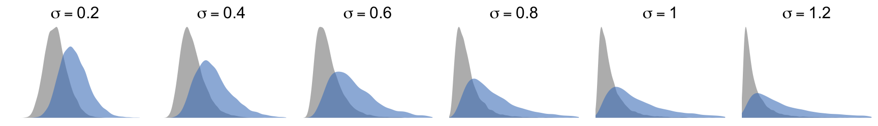
3 Log-normal distributions
In a different experiment, we evaluate log-normal distributions with a wider range of \(\sigma\) parameters (see Figure 6), in particular distributions with less variance, which exhibit a lower degree of skew.
Main effects. Figure 7 presents our results on Type I error rates for main effects. As expected, ART’s inflation of error rates is less serious when distributions are closer to normal, while the problem becomes worse as distributions are more skewed.
Interaction effects. We observe similar patterns for the Type I error rate of the interaction effect in the presence of a single main effect.
Interactions under parallel main effects. We also present results when the two main effects increase in parallel. These results require again careful interpretation, as the null hypothesis of interest may be different for each method. It is important to note that even slight departures from normality (e.g., when \(\sigma = 0.2\)) make the interpretation of interactions problematic.
Conclusion
ART’s robustness issues become less severe as log-normal distributions become less skewed and approach normality. However, interpretation issues for interactions (in the presence of parallel main effects) can arise even when distributions are only slightly skewed.
4 Log-normal distributions with equal variances
As we explain in the article, skewed distributions naturally lead to unequal variances, with the standard deviation of response times typically proportional to the mean. Since ART confounds effects under conditions of unequal variance, an important question remains: Does ART’s difficulty with continuous skewed distributions stem solely from issues of heteroscedasticity?
To address this, we present results from an additional experiment using log-normal distributions in which we directly control the population parameters of the observed distributions (rather than those of the latent variable) to ensure constant variances. Specifically, given a mean \(\mu\) and a fixed standard deviation \(\sigma\) for the responses, the corresponding parameters of the log-normal distribution are:
\(\sigma_{log} = \sqrt{log(1 + \frac{\sigma^2}{\mu^2})}\) and \(\mu_{log} = \log(\frac{\mu^2}{\sqrt{\sigma^2 + \mu^2}})\)
We again consider a \(4 \times 3\) within-subjects design with \(n = 20\), setting the main effect of the first factor to \(a_1 = 2\). We then measure the Power (effect of \(X_1\)) and Type I error rates (effects \(X_2\) and \(X_1 \times X_2\)) of the methods across three standard deviations: \(\sigma = 1\), \(\sigma = 2\), and \(\sigma = 3\).
The following table presents our results. Once again, ART inflates Type I error rates for both the effect of \(X_2\) and its interaction with \(X_1\), with error rates increasing as the common standard deviation grows. In contrast, PAR shows a loss in statistical power, while RNK and INT remain robust.
Table 1: Percentage of positives (%) over 5000 repetitions (\(\alpha = .05\)). For \(X_1\), values reflect statistical power. For \(X_2\) and \(X_1 \times X_2\), they represent Type I error rates.
| PAR | RNK | INT | ART | |
|---|---|---|---|---|
| \(X_1\) | 100 | 100 | 100 | 100 |
| \(X_2\) | 5.0 | 4.9 | 5.4 | 7.6 |
| \(X_1\times X_2\) | 3.6 | 4.2 | 4.6 | 5.7 |
| PAR | RNK | INT | ART |
|---|---|---|---|
| 98.8 | 100 | 100 | 100 |
| 4.0 | 5.1 | 5.3 | 12.1 |
| 3.5 | 5.3 | 5.1 | 9.3 |
| PAR | RNK | INT | ART |
|---|---|---|---|
| 94.0 | 100 | 100 | 100 |
| 3.6 | 4.4 | 4.7 | 17.8 |
| 3.0 | 4.7 | 5.0 | 11.2 |
Conclusion
Heteroscedasticity alone cannot explain ART’s failures under log-normal distributions. ART’s alignment method is based on the assumption that the shape of the distribution (log-normal here) is identical across all factor levels. This is not the case in the above scenarios where distribution shapes change across the levels of \(X_1\), causing the method to break down.
5 Binomial distributions
We also evaluate a wider range of parameters for the binomial distribution. We focus on the lower range of probabilities \(p\). However, we expect results to be identical for their symmetric probabilities \(1-p\). Specifically, we test \(p=.05\), \(.1\), and \(.2\), and for each, we consider \(k=5\) and \(10\) task repetitions (Bernoulli trials).
Main effects. We present our results for the main effect in Figure 10. We observe that ART’s Type I error rates increase as the number of repetitions decreases and the probability of success approaches zero, reaching very high levels when \(k=5\) and \(p=.05\). This trend is consistent across designs. The other methods maintain low error rates. However, their error rates fall below nominal levels when the magnitude of the effect on \(X_1\) grows beyond a certain threshold, indicating a loss of power in these cases.
Interaction effects. Figure 11 shows similar patterns for the Type I error rate of the interaction effect in the presence of a single main effect.
Interactions under parallel main effects. When both main effects exceed a certain level (see Figure 12), all methods fail to control the Type I error rate. Whether this inflation is due to interpretation issues or to a lack of robustness in the methods themselves, these results once again highlight that testing interactions in such scenarios is highly problematic.
Conclusion
ART is extremely problematic under binomial distributions, raising Type I error at very high levels even when effects are null across all factors. We also observe that testing interactions in the presence of parallel main effects can be problematic for all other methods.
6 Ordinal data
Given the frequent use of ART with ordinal data, we evaluate our complete set of ordinal scales, based on both equidistant and flexible thresholds, with additional experimental designs.
Main effects. Figure 13 presents Type I error rates for the main effect. ART preserves error rates at nominal levels under the \(2 \times 3\) between-subjects design and the \(2 \times 3\) mixed design, as long as thresholds are equidistant. Under the two within-subject designs, it inflates error rates, especially when there are fewer ordinal levels with flexible thresholds.
Interaction effects. We present Type I error rates for the interaction effect in the presence of a single main effect. These results lead to similar conclusions. Even in cases where ART keeps error rates close to nominal levels (e.g., under the between-subjects design with equidistance thresholds), the performance of PAR is constantly better.
Interactions under parallel main effects. Finally, we show results for scenarios where main effects increase in parallel.
Conclusion
ART’s inflation of Type I error rates with ordinal data is confirmed across a range of designs. For the between-subjects and mixed designs, the problem primarily concerns ordinal scales with flexible thresholds. For the within-subjects designs, ART also inflates error rates for scales with equidistant thresholds, particularly when the number of levels is as low as five or seven. Again, all methods may fail to correctly infer interactions when parallel main effects exceed a certain threshold.
7 Main effects in the presence of interactions
In all experiments assessing Type I error rates reported in our article, we assumed no interaction effects. However, we also need to understand whether weak or strong interaction effects could affect the sensitivity of the methods in detecting main effects. Unfortunately, the interpretation of main effects may become ambiguous when interactions are present.
Illustrative example
To understand the problem, let us take a dataset from a fictional experiment (within-participants design with \(n = 24\)) that evaluates the performance of two techniques (Tech A and Tech B) under two task difficulty levels (easy vs. hard). Figure 16 visualizes the means for each combination of the levels of the factors, using the original scale of measurements (left) and a logarithmic scale (right). Note that time measurements were drawn from log-normal distributions.
We observe a clear main effect of Difficulty and a strong interaction effect, regardless of the scale. However, the main effect of Technique largely depends on the scale used to present the results. Can we then conclude that Technique A is overall faster than Technique B?
Below, we present the results of the analysis using different methods.
| PAR | LOG | ART | RNK | INT | |
|---|---|---|---|---|---|
| Difficulty | \(7.8 \times 10^{-8}\) | \(4.3 \times 10^{-16}\) | \(8.6 \times 10^{-12}\) | \(2.5 \times 10^{-16}\) | \(1.1 \times 10^{-15}\) |
| Technique | \(.024\) | \(.81\) | \(.00017\) | \(.69\) | \(.69\) |
| Difficulty \(\times\) Technique | \(7.6 \times 10^{-6}\) | \(4.1 \times 10^{-9}\) | \(9.4 \times 10^{-8}\) | \(1.1 \times 10^{-9}\) | \(1.3 \times 10^{-9}\) |
PAR detects a main effect of Technique (\(\alpha = .05\)), as does ART, which yields an even smaller \(p\)-value. In contrast, LOG, RNK, and INT do not find no evidence for such an effect. As with removable interactions, we can speak about removable main effects in this case.
As a general principle, it makes little sense to interpret main effects when crossing patterns emerge due to a strong interaction. In this scenario, the researchers should instead compare techniques within each level of Difficulty. Accordingly, we can conclude that Technique A is slower on easy tasks but faster on hard tasks in this experiment.
Experiment
To better understand how the different methods detect main in the presence of interactions, we conduct an experiment.
We focus again on two-factor experimental designs, setting the sample size to \(n = 20\). To simulate populations in which interactions emerge in the absence of main effects, we examine perfectly symmetric cross-interactions. To this end, we slightly change the method we use to encode the levels of each factor, such that levels are uniformly positioned around 0. For a factor with three levels, we numerically encode the levels as \(\{-0.5, 0, 0.5\}\). For a factor with four levels, we encode them as \(\{-0.5, -0.1667, 0.1667, 0.5\}\).
Since the interpretation of main effects can be ambiguous, we define Type I errors with respect to the coefficients of the linear model. Accordingly, the null hypothesis is either \(a_1 = 0\) or \(a_2 = 0\), depending on the variable of interest.
Interaction effect only. We first examine how the interaction effect alone influences the Type I error rate for \(X_2\). The results are shown in Figure 17. We emphasize that interpretation issues arise only in the case of the \(4 \times 3\) design. In the other two designs, \(X_1\) has only two levels, and due to their symmetry, the observed main effects should be null — regardless of how we define the null hypothesis.
In the \(4 \times 3\) design, error rates for PAR and ART grow rapidly as the interaction effect becomes large under the log-normal and exponential distributions. This is largely due to interpretation issues, as illustrated in our example. However, ART also fails to control the error rate in other scenarios. Finally, under the binomial and ordinal scales, we observe that RNK and INT may also inflate Type I error rates when the interaction effect becomes sufficiently large.
We also examine error rates for the main effect of \(X_2\). Now, interpretation issues affect the results across all three designs, leading to similar patterns.
Interaction effect combined with main effect. Finally, we evaluate the Type I error rate on \(X_2\) when the interaction effect is combined with a main effect on \(X_1\). Figure 19 presents our results.
The error rates of ART and PAR now increase dramatically across all non-normal distributions and all three designs — a result that is, in part, due to interpretation issues. RNK and INT are also affected: their error rates become extremely low under continuous distributions, suggesting a lack of power to detect small main effects when strong effects of other factors are combined with strong interactions. In contrast, under the binomial and ordinal scales, both methods exhibit inflated Type I error rates. Interestingly, RNK demonstrates the best overall performance in these tests.
Conclusion
When strong interactions are present, the interpretation of main effects can become ambiguous, especially when the interaction is combined with a non-zero main effect. ART is more sensitive to these issues than other methods and may even inflate Type I error rates in scenarios where interpretation problems are not expected. More broadly, main effects should be interpreted with caution in the presence of strong interactions.
8 ART with median alignment
We evaluate a modified implementation of ART (ART-MED), where we use medians instead of means to align ranks. This approach draws inspiration from results by Salter and Fawcett (1993), showing that median alignment corrects ART’s instable behavior under the Cauchy distribution. We only test the \(4 \times 3\) within-participants design for sample sizes \(n=10\), \(20\), and \(30\). For this experiment, we omit the RNK method and only present results for non-normal distributions.
We emphasize that Salter and Fawcett (1993) only apply mean and median alignment to interactions. Our implementation for main effects is based on the alignment approach of Wobbrock et al. (2011), where we simply replace means by medians — we are not aware of more adapted methods.
Main effects. Our results presented in Figure 20 demonstrate that median alignment (ART-MED) — or at least our implementation of the method — is not appropriate for testing main effects. Although Type I error rates are now lower for the Cauchy distribution compared to the original method, they are still above nominal levels. In addition, they are significantly higher for all other distributions.
Interaction effects. In contrast, median alignment works surprisingly well for interactions, correcting deficiencies of ART, especially when main effects are absent or weak. Despite this improved performance, we cannot recommend using the method because it still cannot compete with INT. Additionally, its advantages over parametric ANOVA are only apparent for the Cauchy distribution.
Interactions under parallel main effects. We also evaluate Type I error rates for interactions in the presence of parallel main effects, where we caution readers about intepretation issues. We observe again that median alignment improves ART’s bevahior across all distributions. However, as with PAR, its definition of the null hypothesis aligns with the scale of responses rather than with the model parameters.
Conclusion
Using median instead of mean alignment in ART significantly improves the method’s performance for testing interactions across all the distributions we examined. However, we cannot recommend it, as ART remains less robust than INT, and its advantages over PAR are unclear. Moreover, it is not evident how to apply median alignment for testing main effects — using medians with the alignment procedure of Wobbrock et al. (2011) leads to extremely high error rates.
9 Nonparametric tests in single-factor designs
We compare PAR, RNK, and INT to nonparamatric tests for within- and between-subjects single-factor designs, where the factor has two, three, or four levels. Depending on the design, we use different nonparametric tests. For within-subjects designs, we use the Wilcoxon sign-rank test if the factor has two levels (2 within) and the Friedman test if the factor has three (3 within) or four (4 within) levels. For between-subjects designs (2 between, 3 between, and 4 between), we use the Kruskal–Wallis test. We emphasize that alignment procedures are not relevant to single-factor designs. In such cases, the results of ART are identical to those of RNK.
Power. Figure 23 compares the power of the various methods as the magnitude of the main effect increases, where we use the abbreviation NON to designate a nonparametric test. We observe that primarily INT, but also RNK, generally exhibit better power than the nonparametric tests. Differences are more pronounced for within-subjects designs, corroborating Conover’s (2012) observation that the rank transformation results in a test that is superior to the Friedman test under certain conditions.
We expect that the accuracy of ANOVA on rank-transformed values will decrease with smaller samples. However, our tests with smaller samples of \(n=10\) show that INT remains robust and still outperforms other nonparametric methods. Although it is possibe to couple INT with permutation testing for higher accuracy (Beasley, Erickson, and Allison 2009), we have not explored this possibility here.
Type I error rate under equal and unequal variances. Figure 24 presents the rate of positives under conditions of equal (\(r_{sd} = 0\)) and unequal variances (\(r_{sd} > 0\)). While this rate can be considered a Type I error rate when variances are equal, interpreting it under other conditions requires special attention because the hypothesis of interest may differ among methods. Parametric ANOVA is particularly sensitive to unequal variances when distributions are skewed because it tests differences among means. While the normal distributions of the latent space have the same means, this is not the case with the skewed distributions of the transformed variable, which have the same median but different means. All nonparametric methods we tested use ranks, which preserve medians and mitigate this problem. However, their rate of positives can still exceed \(5\%\) under certain conditions.
For between-subjects designs, we observe that the Kruskal–Wallis test and RNK yield very similar results. This is not surprising, as RNK is known to be a good approximation of the Kruskal–Wallis test (Conover 2012). INT’s positive rates are similar, although slightly higher under the binomial distribution. For within-subjects designs, differences among methods are more pronounced. The Wilcoxon sign-rank test (2 within) inflates rates well above \(5\%\), demonstrating that the test is not a pure test of medians. In contrast, the Friedman test (3 within and 4 within) provides the best control among all methods.
Figure 25 presents the same results but for \(\alpha = .01\). Discrepancies among different methods are now more pronounced, and we notice again that the Friedman test keeps rates closer to the nominal level of \(1\%\) compared to INT and RNK. Nevertheless, in addition to their greater power compared to the Friedman test, RNK or INT present other advantages, such as the possibility to use common ANOVA-based procedures to partly correct issues associated with unequal variances. For instance, we ran an experiment, where we applied a Greenhouse–Geisser correction following sphericity violations detected with the Mauchly’s sphericity test (\(\alpha = .05\)). We found that this correction brings the error rates of INT close to nominal levels for continuous distributions, such as the normal and log-normal distributions. In the case of the binomial and ordinal distributions, error rates are also significantly reduced, well below those of the Friedman test, although not reaching nominal levels.
Conclusion
We do not see significant benefits in using dedicated nonparametric tests over RNK or INT. INT can replace nonparametric tests even for single-factor designs. If, after transforming the data, the assumptions of homoscedasticity or sphericity are still not met, applying common correction procedures (e.g., a Greenhouse–Geisser correction for sphericity violations) on the transformed data can reduce the risk of Type I errors.
10 ANOVA-type statistic (ATS)
We compare PAR, RNK, and INT to the ANOVA-type statistic (ATS) (Brunner and Puri 2001) for two-factor designs. We use its implementation in the R package nparLD (Noguchi et al. 2012), which does not support between-subjects designs. Thus, we only evaluate it for the \(4 \times 3\) within-subjects and the \(2 \times 4\) mixed designs.
Type I error rates: Main effects. Figure 26 presents Type I error rates for the main effect of \(X_2\). Under the mixed design, RNK, INT, and ATS exhibit very similar error rates, which are close to nominal levels. In the within-subjects design, the error rates of ATS tend to be slightly above \(5\%\). Additionally, unlike the other methods whose error rates drop significantly below \(5\%\) when the effect of \(X_1\) becomes stronger under binomial and ordinal scales, the power of ATS does not seem to be affected in these cases.
Figure 27 presents results for the main effect of \(X_1\). The error rates of ATS are now slightly inflated under the mixed design. The other methods exhibit the same trends as for the other factor.
Type I error rates: Interactions. Figure 28 presents Type I error rates for the interaction in the presence of a single main effect. Results are again very similar for all three nonparametric methods under the mixed design. In contrast, the error rates of ATS tend to be lower than nominal levels under the within-subjects design, often falling below \(4\%\).
When two parallel main effects are present, ATS and RNK lead to very similar trends (see Figure 29). Overall, INT appears to be a more robust method with the exception of the binomial distribution, for which error rates are higher for this method.
Power: Main effects. As shown in Figure 30 and Figure 31, ATS appears as the most powerful method for detecting effects of \(X_1\) for the mixed design. However, in all other situations, it has less power than INT and offer less power than RNK.
Power: Interactions. Figure 32 shows results on power for interactions. INT emerges again as the most powerful method. The power of ATS is particularly low under the within-subjects design.
Conclusion
Although ATS appears to be a valid alternative, it does not offer clear performance advantages over INT, which is also simpler and more versatile.
11 Generalizations of nonparametric tests
Finally, we evaluate the generalizations of nonparametric tests recommended by Lüpsen (2018, 2023) as implemented in his np.anova function (Lüpsen 2021). Specifically, we evaluate the generalization of the van der Waerden test (VDW), and the generalization of the Kruskal-Wallis and Friedman test (KWF). Their implementation uses R’s aov function and requires considering random slopes in the error term of the model, that is, using Error(s/(x1*x2)) for the two-factor within-participants design and Error(s/x2) for the mixed design, where s is the subject identifier variable. We also used the aov function and the same formulation of the error term for all other methods.
Type I error rates: Main effects. Figure 33 presents Type I error rates for the main effect of \(X_2\). While all methods perform well under the within-subjects and mixed designs, the error rates of VDW and KWF drop drastically as the effect of \(X_1\) grows under the between-subjects design. We will see below that the power of these methods evaporates in these cases.
Type I error rates: Interactions. Figure 34 presents the Type I error rates for the interaction, in the presence of a single main effect. Once again, the error rates of VDW and KWF decrease rapidly in both the between-subjects and mixed designs. Figure 35 shows the results when both main effects are present. Under the within-subjects design, KWF is the poorest-performing technique. While VDW outperforms RNK, it remains inferior to INT. For the between-subjects and mixed designs, KFW and VDW yield low or near-zero error rates when main effects are large, likely due to their extreme loss of power in these scenarios.
Power: Main effects. Figure 36 presents power results for detecting the main effect of \(X_1\). For the within-subjects and mixed design, KFW and VDW exhibit a lower power than RNK and INT, but differences are generally small. Although VDW appears as powerful as INT under the between-subjects design, this only occurs when the effect of the second factor is zero. As shown in Figure 37, the power of both KFD and VDW drops drastically as the effect of \(X_2\) increases for this design.
Figure 38 also presents results for the main effect of \(X_1\), where we observe once again that the generalized tests cannot compete with the more powerful INT, or even with RNK.
Power: Interactions. We also present results on the power of methods to detect interactions in Figure 39, confirming the advantage of INT across all designs. Figure 40 provides a clearer picture of how power is affected by the presence of a main effect. We observe that the power of all methods drops as the main effect of \(X_2\) increases, but this trend is more pronounced for KFD and VDW, particularly for the between-subjects and mixed designs.
Conclusion
Our results do not support Lüpsen’s (2018, 2023) conclusions. The behavior of the generalized nonparametric tests presents issues in numerous scenarios. While these tests exhibit lower error rates under specific conditions, this is due to a significant loss of power when other effects are at play. Therefore, we advise against the use of these methods.
References
Beasley, T Mark, Stephen Erickson, and David B Allison. 2009. “Rank-Based Inverse Normal Transformations Are Increasingly Used, but Are They Merited?” Behav Genet 39 (5): 580–595. https://doi.org/10.1007/s10519-009-9281-0.
Brunner, Edgar, and Madan L. Puri. 2001. “Nonparametric Methods in Factorial Designs.” Statistical Papers 42 (1): 1–52. https://doi.org/10.1007/s003620000039.
Conover, W. Jay. 2012. “The Rank Transformation—an Easy and Intuitive Way to Connect Many Nonparametric Methods to Their Parametric Counterparts for Seamless Teaching Introductory Statistics Courses.” WIREs Computational Statistics 4 (5): 432–438. https://doi.org/10.1002/wics.1216.
Lüpsen, Haiko. 2018. “Comparison of Nonparametric Analysis of Variance Methods: A Vote for van Der Waerden.” Communications in Statistics - Simulation and Computation 47 (9): 2547–2576. https://doi.org/10.1080/03610918.2017.1353613.
Lüpsen, Haiko. 2021. R Code for Nonparametric Procedures. Https://www.uni-koeln.de/~a0032/R.
Lüpsen, Haiko. 2023. “Generalizations of the Tests by Kruskal-Wallis, Friedman and van Der Waerden for Split-Plot Designs.” Austrian Journal of Statistics 52 (5): 101–130. https://doi.org/10.17713/ajs.v52i5.1545.
Noguchi, Kimihiro, Yulia R. Gel, Edgar Brunner, and Frank Konietschke. 2012. “nparLD: An r Software Package for the Nonparametric Analysis of Longitudinal Data in Factorial Experiments.” Journal of Statistical Software 50 (12): 1–3. https://doi.org/10.18637/jss.v050.i12.
Salter, K. C., and R. F Fawcett. 1993. “The Art Test of Interaction: A Robust and Powerful Rank Test of Interaction in Factorial Models.” Communications in Statistics - Simulation and Computation 22 (1): 137–153. https://doi.org/10.1080/03610919308813085.
Wobbrock, Jacob O., Leah Findlater, Darren Gergle, and James J. Higgins. 2011. “The Aligned Rank Transform for Nonparametric Factorial Analyses Using Only Anova Procedures.” Proceedings of the SIGCHI Conference on Human Factors in Computing Systems (New York, NY, USA), CHI ’11, 2011, 143–146. https://doi.org/10.1145/1978942.1978963.